 | Content Disclaimer Copyright @2020. All Rights Reserved. |
StatsToDo: Backpropagation Neural Network
Links : Home Index (Subjects) Contact StatsToDo
|
Explanations
This page provides the program and explanations for the basic Backpropagation Neural Net.
Calculations
Neural net is a vast subject, and subjected to rapid development in the 21st century, as it forms the basis of machine learning and artificial intelligence, and backprpagation is one of the earliest to develop, and form the basic framework for many algorithms. Backpropagation began as a simple adaptive learning algorithm, and this is presented in this page, in the form of a Javascript program, so that users can use the program directly, or if required, copy and adapt the algorithm into their own programs. The program is best viewed as a form of non-parametric regression, where the variables are based on Fuzzy Logic, a number between 0 (false) and 1 (true). Fuzzy Logic The Greek philosopher, Aristotle, stated that things can be true or not true, but cannot be both. Fuzzy logic replaces this statement with that true and false are only extremes that seldom exist, while reality is mostly somewhere in between.
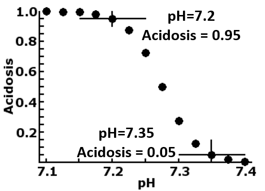
An example of this is shown in the plot to the right, which translates the measurement of fetal blood pH into a diagnosis of acidosis, by firstly rescale the normally accepted non-acidosis value of 7.35 to -2.4444 and its logistic value of 0.05 and the normally accepted acidosis value of 7.2 to 2.4444 and its logistic value of 0.95. This rescaling changes an otherwise normally distributed measurement into the bimodal one of acidosis and non-acidosis, compressing the values less than 7.2 and more then 7.35, while stretches the values in between. Neurone The processing unit in a Backpropagation neuronet is the perceptron, based on the concept of the nerve cell the neurone. The unit receives one or more inputs (dendrites), process them to produce an output (axon). Mathematically, this is divided into two processes.
Neuronet and Backpropagation
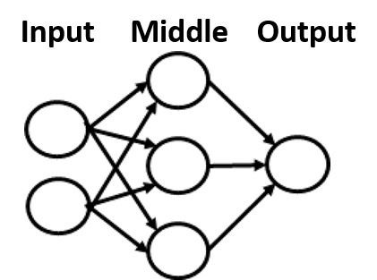
The Backpropagation neuronet is an arrangement of neurones as shown to the right, and consists of the following
Tranining the neuronet The coefficients (w and c) in all of the neurones in a backpropagation neuronet consist of random numbers when the neuronet is initially constructed. Training consists of presenting a series of templates (input and output) to the neuronet, which adapts (learn) through the following processes
Using the trained neuronet At the end of training, the set of coefficients represents the "memory" that has been trained, and can be use to produce outputs from sets of input. Simple neuronet can be process manually, but usually the set of coefficients is incorporated into a computer program or hardwired into machineries. From the Javascript program in this page, the trained neural network can be presented as a program (html and Javascript code) that the user can copy to a text editor and saved as an html file. The html propgram can then be used to interpret future data ReferencesUsers should be aware that neural network generally, and backpropagation in particular, have undergone dramatic development in the 21st century, and the current complexity and capability of these algorithms greatly exceed the content of this page. The program on this page is a simple and primitive one, and can probably used for diagnostic or therapeutic decision making in clearly defined clinical domains, with 5-20 inputs,10-20 patterns to learn, and training dataset of no more than a few hundred templates. It is insufficient to process complex patterns that requires large datasets such as in predicting share prices, company profitability, or weather forecast. where ambiguous data, multiple causal input and output, unknown patterns, and massive training data are involved. The following are references for beginners. They introduce the concept, and lead to further reading. Mueller J P and Massaron L (2019) Deep Learning for Dummies. John Wiley and Sons, Inc., New Jersey. ISBN 978-1-119-54303-9. Chapter 7 and 8 p.131-162. A very good introduction to neuronet and Backpropagation On Line
Hints and Suggestions
R Codes
This panel explains how the program in the program panel can be run, and provides some suggestions on how to make the program run efficiently
Javascript Program
The Structure This is a column of numbers which represents the number of neurones for each layer. The minumum is 2 rows, input and output. The most common is 3 rows, with a single middle layer. In theory there can be any number of middle layers, and there can be any number of neurones in each layer. The following general approach can be used, although each network is unique, and some trial and error may be necessary
The values representing the structure are placed in the Network Structure text area. In our example, there are 3 inputs and one output. The middle layer contains 4 neurones. Data : Input and Output The data is a table of numbers representing the template pattern. It can have any number of rows, but the number of columns is the number of inputs (first row in structure) plus the number of outputs (last row in the structure). For training, the number of columns must conformed to input + output. To use a trained net to interpret a set of data, only the input columns are required. All data used by the backpropagation, be they input parameters or result output, represents Fuzzy Logic, and numerically represented as values between 0 for false, and 1 for True. Real data will therefore need to be edited to conform with this. Fuzzy Logic is discussed in the introduction panel, and will not be elaborated here.
Training Schedule These are parameters that controls the speed and precision of training the neural network. They do not matteer much when the training data is brief, conceptually clear, and all the values are close to 0 and 1 (as in the example). They become increasingly important when the training data is large, where the values are heterogenous, and when the same set of inputs are linked to different outcomes
The neural net text area contains the neural net, a table of coefficients, each row containing the coefficients of a neurone. When the program begins, this area is blanked, as no neural network as yet exists, and the program creates the neural net using random numbers. If the neural net already exists, either because the user paste it in the text area, or if some training has already occurs, the coefficients are used and further modified if more training is performed The program produces coefficients to 10 decimal places, in excess to precision requirements in most cases, but allowing users to truncate them as preferred. In general, the number of decimal places should be 1 or 2 more than the precision of results required by the user. In our example, truncation coefficients to 3 decimal places will produce the same results. The Default Example The default example is a backpropagation network with 3 layers
Suggestions for training The following schedules are suggested to help users not familiar with the program
Using the Trained Neural Net This page also provides a platform for using the Bckpropagation network once it is trained.
Exporting the Trained Neural Net The trained neural net can be exported as a html program
Data Matrix
Neural Net Matrix Using the Trained neural NetUsing the structure, input data and trained neural netCalculate output from information in Structure, input data, and neural net text areas Translate Neural Net as Javascript Program
The R code on this panel is based on the nnet library from https://www.rdocumentation.org/packages/nnet/versions/7.3-16/topics/nnet. The algorithm supports backpropagation calculations for any number of inputs and outputs, but only allows 1 middle layer with any number of neurones.
If more than 1 middle layer is required, user can go to https://cran.r-project.org/web/packages/neuralnet/index.html to download the package neuralnet and its instructions pdf file. The following 2 examples calculates a simple backpropagation neural network The Data: consists of a matrix of 8 rows, with 3 inputs (I1, I2, and I3) and 2 outputs (O1 and O2). After the data frame is created, the library nnet is then called.
myDat = ("
I1 I2 I3 O1 O2
0  0  0  0  1
0  1  0  1  0
1  0  0  1  0
1  1  0  0  1
0  0  1  1  0
0  1  1  0  1
1  0  1  0  1
1  1  1  1  0
")
myDataFrame <- read.table(textConnection(myDat),header=TRUE)
myDataFrame
library(nnet)
Test 1input=I1,I2,I3, 1 middle layer with 4 neurones, output = O1, tolerance=0.05, maximum interation=200x<-subset(myDataFrame, select=I1:I3) #subset x=I1,I2,I3 x y<-c(myDataFrame$O1) #subset y=O1 y nn <- nnet(x,y, size=4, abstol=0.05, maxit = 200) // backpropagation summary(nn) predict(nn)The subset x consists of the 3 inputs I1 to I3. y the single output O1 The function nnet is called.
> x
  I1 I2 I3
1  0  0  0
2  0  1  0
3  1  0  0
4  1  1  0
5  0  0  1
6  0  1  1
7  1  0  1
8  1  1  1
> y<-c(myDataFrame$O1)                     #subset y=O1
> y
[1] 0 1 1 0 1 0 0 1
> nn <- nnet(x,y, size=4, abstol=0.05, maxit = 200)
# weights:  21
initial  value 2.050771
iter  10 value 1.999513
iter  20 value 1.913413
iter  30 value 1.597108
iter  40 value 0.216418
final  value 0.033959
converged
> summary(nn)
a 3-4-1 network with 21 weights
options were -
 b->h1 i1->h1 i2->h1 i3->h1
  2.16  -5.72  -0.09   1.12
 b->h2 i1->h2 i2->h2 i3->h2
  5.10  -1.99  -4.27  -4.27
 b->h3 i1->h3 i2->h3 i3->h3
  2.64  -1.68   1.87   5.01
 b->h4 i1->h4 i2->h4 i3->h4
 -4.91  -9.70  10.28   9.01
 b->o h1->o h2->o h3->o h4->o
-3.18 -6.82  7.57 -0.95  7.93
> predict(nn)
        [,1]
1 0.06983661
2 0.95256979
3 0.96103373
4 0.08941800
5 0.91531074
6 0.07498991
7 0.05624830
8 0.96314380
newDat = ("
          I1  I2  I3
          0.1 0.2 0.05
          0.3 0.9 0.0
          0.8 0.1 0.1
          ")
newData<-read.table(textConnection(newDat),header=TRUE)
predict(nn, newData)
The results are
> predict(nn, newData)
          [,1]
[1,] 0.1086763
[2,] 0.9636761
[3,] 0.9212004
Test 2This is the same as test 1, except that there are now 2 outputs O1 and O2.The program is x<-subset(myDataFrame, select=I1:I3) #subset x=I1,I2,I3 x y<-subset(myDataFrame, select=O1:O2) #subset y=O1,O2 y nn <- nnet(x,y, size=4, abstol=0.05, maxit=200) summary(nn) predict(nn)The results are
> x
  I1 I2 I3
1  0  0  0
2  0  1  0
3  1  0  0
4  1  1  0
5  0  0  1
6  0  1  1
7  1  0  1
8  1  1  1
> y<-subset(myDataFrame, select=O1:O2)     #subset y=O1,O2
> y
  O1 O2
1  0  1
2  1  0
3  1  0
4  0  1
5  1  0
6  0  1
7  0  1
8  1  0
> nn <- nnet(x,y, size=4, abstol=0.05, maxit=200)
# weights:  26
initial  value 4.071980
iter  10 value 3.999929
iter  20 value 3.990630
iter  30 value 1.902310
final  value 0.037599
converged
> summary(nn)
a 3-4-2 network with 26 weights
options were -
 b->h1 i1->h1 i2->h1 i3->h1
 -1.96  -2.40   0.04   0.15
 b->h2 i1->h2 i2->h2 i3->h2
 12.68  65.74 -40.83 -65.08
 b->h3 i1->h3 i2->h3 i3->h3
  3.57   3.40  -0.89  -2.10
 b->h4 i1->h4 i2->h4 i3->h4
 -0.58  -1.89   4.56   2.13
 b->o1 h1->o1 h2->o1 h3->o1 h4->o1
 -0.32  -7.82 -16.71  20.34 -15.00
 b->o2 h1->o2 h2->o2 h3->o2 h4->o2
  1.63   7.85  17.30 -22.59  15.04
> predict(nn)
            O1          O2
1 2.689003e-02 0.965504577
2 9.521576e-01 0.023248336
3 8.834675e-01 0.086618520
4 3.778867e-05 0.999949062
5 9.400405e-01 0.038104978
6 3.346196e-02 0.963676744
7 3.884451e-02 0.948116245
8 9.914175e-01 0.003671725
There are now two outputs O1 and O2.
As with Test 1, the trained neural net is tested on a new set of data, and produced two outputs
newDat = ("
          I1  I2  I3
          0.1 0.2 0.05
          0.3 0.9 0.0
          0.8 0.1 0.1
          ")
newData<-read.table(textConnection(newDat),header=TRUE)
predict(nn, newData)
The results are
> predict(nn, newData)
              O1          O2
[1,] 0.001618309 0.997914331
[2,] 0.989863726 0.004413234
[3,] 0.546131182 0.375853575
|
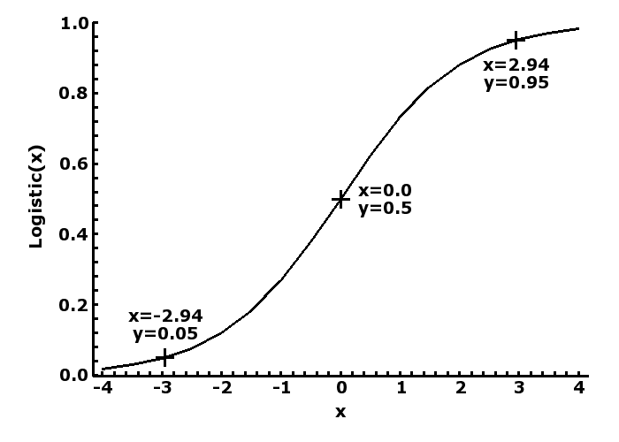
 Mathematically this is represented as a number (y) between 0 (false) and 1 (true), and its relationship to a linear measurement (x) represented by the logistic curve (y = 1/(1+exp(-x)), as shown in the plot to the left, where a value of 0 is translated to a probability of 0.5, -∞ to 0 and or +∞ to 1. If we then accept that <=0.05 as unlikely to be true and >=0.95 likely to be true, then we can rescale any measurement to -2.9444 and + 2.9444, which is then logistically transformed to 0.05 and 0.95. Program for logistic transformation is available at
