Macroplot plotting is controlled by the macros in the text area provided.
Each macro must occupy its own line. If the first character of a macro is not A-Z, the line will be considered a comment and ignored
The first macro, which is obligatory, initializes the plot. The macro is
Bitmap Initialize width(in pixels), height(in pixels), red(0-255) blue(0-255), green(0-255) transparency(0-255)
Example : Bitmap Initialize 700 500 255 255 255 255 which provides a landscape area 700 pixels wide, 500 pixel high, with white background
The following are default settings when the bitmap is initiated.
Lines are black (0 0 0 255) and 3 pixels in width
Fill color for bars and dots are black (0 0 0 255), and the fill type is set to fill only (1) (see Fill Type)
Dots (circl and square) are set to 5 pixels radius (diameter=11 pixels)
Fonts are set as follows
Font face is set to sans-serif. Serif, sans-serif, and monospace are available to all browsers, user can use any font available to his/her browser
Font size is set to 16 pixels high
Font color, both line and fill are set to black (0 0 0 255), and fill type to 1 (fill only) (see Font Type)
Macros for plotting on the bitmap begin with the keyword Bitmap, and the coordinates are x=number of pixels from the left border and y=number of pixels from the top border
A central plotting area is also defined
By default, at initialization, as 15% from the left and bottom, 5% from right and top
defined by user as Plot Pixels left top right bottom, these being number of pixels from the left and top border
e.g. Plot Pixels 105 25 665 425 would be the same as the default setting for a bitmap of 700 pixels wide and 500 pixels high
The values of the data used in plotting in this central area can be defined as follows
Plot Values left top right bottom, these being the extreme values used in the data
e.g.Plot Values 0 100 10 50 represents x values of 0 on the left to 10 to the right, and y values of 50 at the bottom to 100 to the top
After the values are declared, all plotting in the central area uses macros beginning with the keyword Plot, and the coordinates are the values in the data
Macros
This panel lists and describes all macros used in this version of MacroPlot by Javascript. They are divided into the following sub-panels
Initialization and settings
Plotting areas, coordinates used, and drawing of x and y axis
Drawing lines, bars, dots, text, and other shapes
Initialization
This sub-panel lists those macros that initialized the bitmap, and set the parametrs for drawing
Initialize Plotting
Bitmap Initialize w h r g b t is the first and obligatory macro, which Initializes the bitmap
w and h are width and height of the bitmap in number of pixels. The most common dimensions are
w=700 and h= 500 for landscape orientation
w=500 and h=700 for portrait orientation
Both 500 for square bitmap
r g b t represents red, green, blue and transparency values for the background, each value is 0 for non-existence to 255 for maximum intensity. The most commonly used background is white (255 255 255 255)
For most plotting programs in StatsToDo the macro used is Bitmap Initialize 700 500 255 255 255 255, a landscape orientation with white background
Settings for lines
The settings provide parameters for all subsequent plotting until the parameter is reset
Line Color r g b t sets the line color of red, green, blue and transparency values, each value is 0 for non-existence to 255 for maximum intensity. On initialization of the bitmap, line color is lines is set by default to black (0 0 0 255)
Line Thick p sets the thickness of lines to p pixels. On initialiszation, the default setting is 3 pixels for line thickness
Settings for fills
When bars, dots, arcs and wedges are plotted, the interior of these symbols are called fills, and they are set as follows
Fill Color r g b t sets the filling color of red, green, blue and transparency values, each value is 0 for non-existence to 255 for maximum intensity. On initialization of the bitmap, fill color is lines is set by default to black (0 0 0 255).
Fill Type t sets how the fills are to be used, t can be one of the following
t=0: only the outline, defined by the line parameters, are plotted. Fill is ignored
t=1: only fill is carried out, outline is ignored
t=2: both outline and fill are plotted
When the plot is initialized, the default setting for fill type is t=1
Settings for fonts
These set the font characteristics for text output. Please note: settings for lines and fills for fonts are separate and independent to those for general line and shape plottings
Font Face name sets the font face. The program will accept all fonts supported by the user's border. The 3 fonts accepted by all browsers are serif, sans-serif, and monospace. On initialization, sans-serif is set by default
Font Style s where s can be either normal or bold. On initialization the default setting is bold
Font Size h where h is the height of the text in pixels. On initialization, the default font size is set to 16
Font Thick p where p is the thickness of the outline of the font. On initialization, this is set to p=1
Font LColor r g b t sets the color of the outline of the font. On initialization this is set to black (0 0 0 255)
Font FColor r g b t sets the fill color of the of the font. On initialization this is set to black (0 0 0 255)
Font Color r g b t sets both LColor and FColor to the same color. On initialization this is set to black (0 0 0 255)
Font Type t where t determines which part of the font is drawn, and can be one of the following
t=0: only the outline of the font, defined by the thick and LColor parameter is drawn
t=1: only the fill of the font is drawn
t=2: both outline and fill are drawn
When the plot is initialized, the default setting for Font type is t=1
Please Note: When the bitmap is initialized, the default settings, which are suitable for most situations, are automatically set, so users need not worry about these settings unless he/she has a different preference.
Axis & Coordinates
This sub-panel presents macros that define the plotting areas, and creating the x and y axis for plotting
Drawing on the bitmap
When plotting on the initialized bitmap
the horizontal coordinate x is the number of pixels from the left border
the vertical coordinate y is the number of pixels from the top border
The macro used begins with the keyword Bitmap
Drawing on the plotting area
In most cases, there is a need to draw and label the x and y axis, and drawing coordinates used are the actual values of the data. The macros used for these all begins with the keyword Plot, and are purposes are as follows
Plot Pixels lp tp rp bp defines an area for plotting
lp defines the left border of the plotting area, in the number of pixels from the left border of the bitmap. In most cases this is 15% of the bitmap's width
tp defines the top of the plotting area, in the number of pixels from the top border of the bitmap. In most cases this is 5% of the height
rp defines the right border of the plotting area, in the number of pixels from the left border of the bitmap. In most cases this is 95% of the width (or 5% from the right border of the bitmap)
bp defines the bottom border of the plotting area, in the number of pixels from the top border of the bitmap. In most cases this is 85% of the height (or 15% from the bottom)
An example is that is that, in a landscape orientated bitmap of 700 pixels width and 500 pixel height, Plot Pixels 105 25 665 425 sets the central area for plotting that is 15% from the left and bottom, and 5% from the top and right.
This macro is usually not necessary if the 5%/15% setting suits the user, as this is the default setting when the bitmap is initialized
Plot Values lv tv rv bv defines the data values to be used in plotting
lv is the extreme data value for the horizontal variable x on the left
tv is the extreme data value for the vertical variable y at the top
rv is the extreme data value for horizontal variable x on the right
bv is the extreme data value for the vertical variable y at the bottom
Plot Logx 1 sets the horizontal x axis to the log scale. Normal scale is set on initialization, or reset by Plot Logx 0
Plot Logy 1 sets the vertical y axis to the log scale. Normal scale is set on initialization, or reset by Plot Logy 0
Plot XLabel label distance places the label for the horizontal x axis, below the bottom of the plotting area
lable is a single word text string, using the underscore _ to represent spaces if necessary
space is the number of pixels between the bottom of the plot area and the label text string
Plot YLabel label distance places the label for the vertical y axis, on the left of plotting area
lable is a single word text string, using the underscore _ to represent spaces if necessary
space is the number of pixels between the left of the plot area and the label text string
The quickest and easiest way to draw axis
The following 4 macros are sufficient to draw the x and y axis under most circumstances
Plot XAxis y nsIntv nbIntv len gap line will mark out and numerate the horizontal x axis
y is the y value on which the x axis lie
nsIntv is the number of small intervals between the vertical line marks, 10 to 20 are recommended
nbIntv is the number of big intervals between the numerical scales, 5 to 10 are recommended
len is the length of the mark in pixels, +ve value downwards and negative value upwards. -10 is recommended
gap is the number of pixels between the numerical scaling text and the y value of the axis, +ve values for text below axis and negative value for text above axis. 3 is recommended
Line determines the axis line is drawn, 0 for no line, 1 for line
Plot YAxis x nsIntv nbIntv len gap line will mark out and numerate the vertical y axis
x is the x value on which the y axis lie
nsIntv is the number of small intervals between the horizontal line marks, 10 to 20 are recommended
nbIntv is the number of big intervals between the numerical scales, 5 to 10 are recommended
len is the length of the mark in pixels, +ve value to the right and negative value to the left. 10 is recommended
gap is the number of pixels between the numerical scaling text and the y value of the axis, +ve values for text to the right of axis and negative value for text to the left of axis. -3 is recommended
Line determines the axis line is drawn, 0 for no line, 1 for line
Plot AutoXLogScale y len gap line will mark and numerate the x axis if it is in log scale
The x axis must be set to the log scale by Plot Logx 1. If axis not set to log this macro will abort
y is the y value on which the x axis lie
len is the length of the mark in pixels, +ve value downwards and negative value upwards. -10 is recommended
gap is the number of pixels between the numerical scaling text and the y value of the axis, +ve values for text below axis and negative value for text above axis. 3 is recommended
Line determines the axis line is drawn, 0 for no line, 1 for line
Plot AutoYLogScale x len gap line will mark and numerate the y axis if it is in log scale
The y axis must be set to the log scale by Plot Logy 1. If axis not set to log this macro will abort
x is the x value on which the x axis lie
len is the length of the mark in pixels, +ve value downwards and negative value upwards. -10 is recommended
gap is the number of pixels between the numerical scaling text and the y value of the axis, +ve values for text below axis and negative value for text above axis. 3 is recommended
Line determines the axis line is drawn, 0 for no line, 1 for line
Other methods of drawing axis
Users may wish to draw individual part of the axis, and the following macros can be used
Plot XLine y Draws the horizontal x axis line at the y value y
Plot YLine x Draws the vertical y axis line at the x value y
Plot XMark y begin interval len marks the horizontal x axis with a series of vertical marks
y is the y value where the axis is to be marked
begin is the value for the first mark
interval is the interval between marks
len is the length of the mark line in pixels, +ve downwards, -ve upwards
Plot YMark x start interval len marks the vertical y axis with a series of horizontal marks
x is the x value where the axis is to be marked
start is the value for the first mark
interval is the interval between marks
len is the length of the mark line in pixels, +ve to the right, -ve to the left
Plot XScale y start interval gap writes the numerical scales for the horizontal x axis
y is the y value for the axis
start is the first value to be written
interval is the interval between numerical scales
gap is the space in pixels between the scale text and the axis, +ve for text below axis, -ve for text above axis
The number of decimal points in the scale is the same as that of the interval value
Plot YScale x start interval gap writes the numerical scales for the vertical y axis
x is the x value for the axis
start is the first value to be written
interval is the interval between numerical scales
gap is the space in pixels between the scale text and the axis, +ve for text to the right of axis, -ve for text to the left of axis
The number of decimal points in the scale is the same as that of the interval value
Plot XMarkIntv y interval len marks the horizontal x axis with a series of vertical marks
y is the y value of the axis
interval is the interval between the marks, beginning at 0 and while in range
len is the length of the mark line in pixels, +ve downwards, -ve upwards
Plot YMarkIntv x interval len marks the vertical y axis with a series of horizontal marks
x is the x value of the axis
interval is the interval between the marks, beginning at 0 and while in range
len is the length of the mark line in pixels, +ve to the right, -ve to the left
Plot XScaleIntv y interval gap writes the numerical scales for the horizontal x axis
y is the y value of the axis
interval is the interval between the numerical scales, beginning at 0 and while in range
gap is the space in pixels between the scale text and the axis, +ve for text below axis, -ve for text above axis
The number of decimal points in the scale is the same as that of the interval value
Plot YScaleIntv x interval gap writes the numerical scales for the vertical y axis
x is the x value of the axis
interval is the interval between the numerical scales, beginning at 0 and while in range
gap is the space in pixels between the scale text and the axis, +ve for text to the right of axis, -ve for text to the left of axis
The number of decimal points in the scale is the same as that of the interval value
Drawings
This sub-panel describes those macros that draws the plotting objects. Drawing are performed in two environments
Macros that begins with the keyword Bitmap uses pixel values as coordinates, where x is the number of pixels from the left border, and y the number of pixels from the top border
Macros that begins with the keyword Plot uses actual data values (as defined in the Plot Values lv tv rv bv macro, as coordinates
Drawing lines
The thickness and color of any line drawn is set by the Line macros (see setting sub-panel). The default setting is black line 3 pixels in width
Bitmap Line x1 y1 x2 y2 draws the line from x1y1 to x2y2
x1 and x2 are number of pixels from the left border
y1 and y2 are number of pixels from the top border
Plot Line x1 y1 x2 y2 draws the line from x1y1 to x2y2
x1 and x2 are data values for the horizontal variable x
y1 and y2 are data variables for the vertical variable y
Plot PixLine x y hpix vpix draws a line
x and y are data values for the horizonal x value and verticsl y value. This defines the coordinate at the origin of the line
hpix is the number of pixels horizontally from the origin, +ve value to the right, -ve value to the left
vpix is the number of pixels vertically from the origin, +ve value downwards, -ve value upwards
The line is then drawn between the origin and that defined by hpix and vpix
Drawing bars
The color and thickness of the outline are defined in the Line macro. The color of the fill is defined in the fill color and Fill Type macro. The default setting is black (0 0 0 255) for both line and fill color, and the Fill type is set to 1, only the fill and no outlines. These settings are suitable for most circumstances, but user can change them is so required.
Bitmap Bar x1 y1 x2 y2 draws a bar the corner of which are x1y1 and x2y2. X and y are number of pixels from the left and top border of the bitmap
Plot Bar x1 y1 x2 y2 draws a bar the corner of which are x1y1 and x2y2. X and y are data values as defined in Plot Values lv tv rv bv
Bar Wide w sets the width / height of bars for Plot VBar and Plot HBar
w is the half width of the bar, so a VBar is 2w+1 pixels in width, and HBar is 2w+1 pixels in height
The default value for w is 7 pixels (making width/height of 15 pixels), unless the user changes it
Plot VBar x y1 y2 hshift draws a vertical bar
x is the data value for the horizontal x variable. The is the center of the vertical bar
y1 and y2 are values for the vertical y variable. They define the vertical ends of the bar
hshift is the number of pixels the whole bar is shefted horizontally, +ve value to the left and +ve value to the right. In most cases this is 0 (no shift). However, if there are more than 1 bar in the same position, shifting some of them will avoid the bars overlapping and obscuring each other
The width of the vertical bar is set by default at 7, (width of bar=15 pixels)
Plot HBar x1 x2 y vshift draws a horizontal bar
x1 and x2 are data values for the horizontal x variable. They define the horizontal ends of the bar
y is the value for the vertical y variable, and defines and center of the horizontal bar
vshift is the number of pixels the whole bar is shefted vertically, -ve value upwards and +ve value downwards. In most cases this is 0 (no shift). However, if there are more than 1 bar in the same position, shifting some of them will avoid the bars overlapping and obscuring each other
Theheight of the horizontal bar is set by default at 7, (height of bar=15 pixels)
Drawing dots
There are only 2 dot types, circle and square. If more than 2 tyoes of dats are required, they can be distinguished by the colours of the outline and fill, and by their sizes. Settingsd for dot parameters are in the settings sub-panel
Bitmap Circle x y radius and Bitmap Square x y radius draws a circle or a square dot
x and y are the number of pixels from the left and top border
Radius is in number of pixels. The diameter of the dot is 2Radius+1 pixels
Plot Circle x y radius hshift vshift and Plot Square x y radius hshift vshift draws a circle or a square dot
x and y are the data values of the horizontal x variable and vertical y variable, as defined by Plot Values lv tv rv bv
Radius is in number of pixels. The diameter of the dot is 2Radius+1 pixels
hshift is the number of pixels the dot is shifted horizontally, -ve value to the left, +ve value to the right
vshift is the number of pixels the dot is shifted vertically, -ve value upwards, +ve value downwards
In most cases there is no shift (0 0), but id there are more than 1 dot in the same position, shifting avoids the dots superimposing over and obscuring each other
Dot Radius r sets the radius of the dot in pixels. The diameter of the dot is 2radius+1 pixels. The default radius is 5
Dot Type t where t is either circle or square. The default setting is circle
Plot Dot x y hshift vshift draws the dot, with its parameters (shape size color outline fill) already pre-set
x and y are the data values of the horizontal x variable and vertical y variable, as defined by Plot Values lv tv rv bv
hshift is the number of pixels the dot is shifted horizontally, -ve value to the left, +ve value to the right
vshift is the number of pixels the dot is shifted vertically, -ve value upwards, +ve value downwards
In most cases there is no shift (0 0), but if there are more than 1 dot in the same position, shifting avoids the dots superimposing over and obscuring each other
Drawing text
The color, outline, fill, font, and weight of text are preset (see settings). The default settinfs are sans-sherif, black fill only, and 16pxs high
Bitmap HText x y ha va txt draws text horizontally on the bitmap
x and y are number of pixels fom the left and top borders, and together being the reference coordinate of the text
ha is horizontal adjust
ha=0: the left end of the text is at the x coordinate
ha=1: the center of the text is at the x coordinate
ha=2: the right end of the text is at the x coordinate
va is vertical adjust
va=0: the top of the text is at the y coordinate
va=1: the center of the text is at the x coordinate
va=2: the bottom end of the text is at the x coordinate
txt is the text to be drawn. It must be a single word with no gaps. Spaces can be represented by the underscore _
Plot HText x y ha va txt hshift vshift draws text horizontally on the bitmap
x and y are data values as defined by Plot Values lv tv rv bv, and together being the reference coordinate of the text
ha is horizontal adjust
ha=0: the left end of the text is at the x coordinate
ha=1: the center of the text is at the x coordinate
ha=2: the right end of the text is at the x coordinate
va is vertical adjust
va=0: the top of the text is at the y coordinate
va=1: the center of the text is at the x coordinate
va=2: the bottom end of the text is at the x coordinate
txt is the text to be drawn. It must be a single word with no gaps. Spaces can be represented by the underscore _
hshift is the number of pixels the text is shifted horizontally, -ve value to the left, +ve value to the right
vshift is the number of pixels the text is shifted vertically, -ve value upwards, +ve value downwards
In most cases there is no shift (0 0), but if there are other structures in the same position, shifting avoids the text and structures obscuring each other
Bitmap VText x y ha va txt draws text vertically (90 degrees anticlockwise from horizontal) on the bitmap
x and y are number of pixels fom the left and top borders, and together being the reference coordinate of the text
ha is horizontal adjust
ha=0: the left end of the text is at the x coordinate
ha=1: the center of the text is at the x coordinate
ha=2: the right end of the text is at the x coordinate
va is vertical adjust
va=0: the top of the text is at the y coordinate
va=1: the center of the text is at the x coordinate
va=2: the bottom end of the text is at the x coordinate
txt is the text to be drawn. It must be a single word with no gaps. Spaces can be represented by the underscore _
Plot VText x y ha va txt hshift vshift draws text vertically (90 degrees anticlockwise from horizontal) on the bitmap
x and y are data values as defined by Plot Values lv tv rv bv, and together being the reference coordinate of the text
ha is horizontal adjust
ha=0: the left end of the text is at the x coordinate
ha=1: the center of the text is at the x coordinate
ha=2: the right end of the text is at the x coordinate
va is vertical adjust
va=0: the top of the text is at the y coordinate
va=1: the center of the text is at the x coordinate
va=2: the bottom end of the text is at the x coordinate
txt is the text to be drawn. It must be a single word with no gaps. Spaces can be represented by the underscore _
hshift is the number of pixels the text is shifted horizontally, -ve value to the left, +ve value to the right
vshift is the number of pixels the text is shifted vertically, -ve value upwards, +ve value downwards
In most cases there is no shift (0 0), but if there are other structures in the same position, shifting avoids the text and structures obscuring each other
Other miscellaneous drawings
Bitmap Arc x y radius startDeg endDeg rotate draws an arc.
x and y are number of pixels from the left and top border, and together form the center of the arc
radius is the radius of the arc, in number of pixels
startDeg and endDeg are the degrees (360 degrees in full circle) of the arc
rotate defines the direction of the arc, 0 for clockwise, 1 for anti-clockwise
Bitmap Wedge x y radius startDeg endDeg shift rotate draws a wedge, essentially an arc with lines to the center
x and y are number of pixels from the left and top border, and together form the center of the wedge
radius is the radius of the edge, in number of pixels
startDeg and endDeg are the degrees (360 degrees in full circle) of the wedge
shift is the number of pixels that the wedge is moved centrifugally (away from the center). This is used in pie charts to separate the wedges of the pie
rotate defines the direction of the wedge, 0 for clockwise, 1 for anti-clockwise
Plot Curve a b1 b2 b3 b4 b5 x1 x2 draws a polynomial curve
The curve is y=a + b1x + b2x2 + b3x3 + b4x4 + b5x5. Where higher power is not needed, 0 is used to represent the the coefficient b
The curve is drawn from data value x from x1 to x2
Plot Normal mean sd height draws a normal distribution curve
mean and sd (Standard Deviation) are as in the data horizontal variable variable x
height is the maximum height (where x=mean) of the curve as in the vertical variable y
Color Palettes
Plain Colors
0 0 0 #000000
0 0 63 #00003f
0 0 127 #00007f
0 0 191 #0000bf
0 0 255 #0000ff
0 63 0 #003f00
0 63 63 #003f3f
0 63 127 #003f7f
0 63 191 #003fbf
0 63 255 #003fff
0 127 0 #007f00
0 127 63 #007f3f
0 127 127 #007f7f
0 127 191 #007fbf
0 127 255 #007fff
0 191 0 #00bf00
0 191 63 #00bf3f
0 191 127 #00bf7f
0 191 191 #00bfbf
0 191 255 #00bfff
0 255 0 #00ff00
0 255 63 #00ff3f
0 255 127 #00ff7f
0 255 191 #00ffbf
0 255 255 #00ffff
63 0 0 #3f0000
63 0 63 #3f003f
63 0 127 #3f007f
63 0 191 #3f00bf
63 0 255 #3f00ff
63 63 0 #3f3f00
63 63 63 #3f3f3f
63 63 127 #3f3f7f
63 63 191 #3f3fbf
63 63 255 #3f3fff
63 127 0 #3f7f00
63 127 63 #3f7f3f
63 127 127 #3f7f7f
63 127 191 #3f7fbf
63 127 255 #3f7fff
63 191 0 #3fbf00
63 191 63 #3fbf3f
63 191 127 #3fbf7f
63 191 191 #3fbfbf
63 191 255 #3fbfff
63 255 0 #3fff00
63 255 63 #3fff3f
63 255 127 #3fff7f
63 255 191 #3fffbf
63 255 255 #3fffff
127 0 0 #7f0000
127 0 63 #7f003f
127 0 127 #7f007f
127 0 191 #7f00bf
127 0 255 #7f00ff
127 63 0 #7f3f00
127 63 63 #7f3f3f
127 63 127 #7f3f7f
127 63 191 #7f3fbf
127 63 255 #7f3fff
127 127 0 #7f7f00
127 127 63 #7f7f3f
127 127 127 #7f7f7f
127 127 191 #7f7fbf
127 127 255 #7f7fff
127 191 0 #7fbf00
127 191 63 #7fbf3f
127 191 127 #7fbf7f
127 191 191 #7fbfbf
127 191 255 #7fbfff
127 255 0 #7fff00
127 255 63 #7fff3f
127 255 127 #7fff7f
127 255 191 #7fffbf
127 255 255 #7fffff
191 0 0 #bf0000
191 0 63 #bf003f
191 0 127 #bf007f
191 0 191 #bf00bf
191 0 255 #bf00ff
191 63 0 #bf3f00
191 63 63 #bf3f3f
191 63 127 #bf3f7f
191 63 191 #bf3fbf
191 63 255 #bf3fff
191 127 0 #bf7f00
191 127 63 #bf7f3f
191 127 127 #bf7f7f
191 127 191 #bf7fbf
191 127 255 #bf7fff
191 191 0 #bfbf00
191 191 63 #bfbf3f
191 191 127 #bfbf7f
191 191 191 #bfbfbf
191 191 255 #bfbfff
191 255 0 #bfff00
191 255 63 #bfff3f
191 255 127 #bfff7f
191 255 191 #bfffbf
191 255 255 #bfffff
255 0 0 #ff0000
255 0 63 #ff003f
255 0 127 #ff007f
255 0 191 #ff00bf
255 0 255 #ff00ff
255 63 0 #ff3f00
255 63 63 #ff3f3f
255 63 127 #ff3f7f
255 63 191 #ff3fbf
255 63 255 #ff3fff
255 127 0 #ff7f00
255 127 63 #ff7f3f
255 127 127 #ff7f7f
255 127 191 #ff7fbf
255 127 255 #ff7fff
255 191 0 #ffbf00
255 191 63 #ffbf3f
255 191 127 #ffbf7f
255 191 191 #ffbfbf
255 191 255 #ffbfff
255 255 0 #ffff00
255 255 63 #ffff3f
255 255 127 #ffff7f
255 255 191 #ffffbf
255 255 255 #ffffff
Color Palletes
Table of colors used on this web site
255 255 255 #ffffff
224 224 224 #e0e0e0
128 128 128 #808080
128 0 0 #800000
255 0 0 #ff0000
96 48 96 #603060
48 16 64 #301040
96 96 160 #6060a0
160 160 96 #a0a060
160 160 0 #a0a000
153 191 164 #99bfa4
160 160 96 #a0a060
97 24 0 #611800
204 63 200 #cc3fc8
224 224 224 #e0e0e0
Patterns of complementary colors
A
105 93 70 #695d46
255 113 44 #ff712c
207 194 145 #cfc291
161 232 217 #a1e8d9
255 246 197 #fff6c5
B
115 0 70 #730046
201 60 0 #c93c00
232 136 1 #e88801
255 194 0 #ffc200
191 187 17 #bfbb11
C
97 24 0 #611800
140 115 39 #8c7327
71 164 41 #47a429
153 191 164 #99bfa4
242 239 189 #f2efbd
D
20 87 110 #14576e
140 33 90 #8c215a
230 133 38 #e68526
195 102 163 #c366a3
242 207 242 #f2cff2
E
64 1 1 #400101
48 115 103 #307367
96 166 133 #60a685
242 236 145 #f2ec91
229 249 186 #e5f9ba
F
55 89 21 #375915
166 60 60 #a63c3c
115 108 73 #736c49
166 157 129 #a69d81
242 224 201 #f2e0c9
G
115 36 94 #73245e
166 69 33 #a64521
217 182 78 #d9b64e
242 218 145 #f2da91
242 242 242 #f2f2f2
H
255 77 0 #ff4d00
102 87 71 #665747
125 179 0 #7db300
153 138 122 #998a7a
217 195 98 #d9c362
I
128 0 38 #800026
128 128 83 #808053
92 153 122 #5c997a
163 204 143 #a3cc8f
255 230 153 #ffe699
Explanations
This page provides calculations for parametric correlation (Pearsoon) and linear regression analysis
Correlation
Pearson's Correlation coefficient (ρ) is a measure of associatin between two normally distributed measurements. It describes the strength of association, but does not indicate which is cause and which is effect.
In earlier algorithms, ρ is assumed to have an approximate normal distribution, and its Standard Error to be sqrt((1-ρ2) / (n-2)), where n is sample size. From this the t value and statistical significance based on the t distribution can be estimated.
More recently, that the value of ρ is constrained between -1 and 1 is taken into consideration, and that its distribution is only symmetrical when the value is closed to 0. As ρ value approaches the extreme of -1 or 1, the distribution becomes increasingly asymmetrical, with a long tail towards 0 and short tail towards -1 or 1. Significant test based on the t test is therefore considered at best approximate, and possibly misleading, and the confidence interval, calculated after ρ is transformed to the parametric Fisher's Z is considered more appropriate.
The calculations on this page provides both, allowing the user to decide which one to show as results.
The formulae used for Fisher's Z transformation are
Fisher's Z: Z = log((1 + ρ) / (1 - ρ)) / 2
Standard Error of Z: SE = 1.0 / sqrt(n - 3), where n = sample size
95% CI of Z = Z ± z * SE, where z = 1.64 for 1 tail, and z=1.96 for 2 tail
Reverse transformation : ρ = exp(2Z - 1) / exp(2Z + 1)
X val
Y val
RegY
SEYx
95% CI of RegY
ZY
37
3048
2936.0
47.6
2836.8 to 3035.4
2.36
36
2813
2705.7
58.5
2583.7 to 2827.7
1.83
41
3622
3857.2
82.1
3685.9 to 4028.4
-2.86
36
2706
2705.7
58.5
2583.7 to 2827.7
0.01
35
2581
2475.4
74.1
2320.8 to 2630.1
1.42
39
3442
3396.6
51.7
3288.7 to 3504.5
0.88
40
3453
3626.9
65.2
3490.9 to 3762.9
-2.67
37
3172
2936.0
47.6
2836.8 to 3035.2
4.96
35
2386
2475.4
74.1
2320.8 to 2630.1
-1.21
39
3555
3396.6
51.7
3288.7 to 3504.5
3.06
37
3029
2936.0
47.6
2836.8 to 3035.2
1.96
37
3185
2936.0
47.6
2836.8 to 3035.3
5.24
36
2670
2705.7
58.5
2583.7 to 2827.7
-0.61
38
3314
3166.3
44.9
3072.7 to 3259.9
3.29
41
3596
3857.2
82.1
3685.9 to 4028.4
-3.18
38
3312
3166.3
44.9
3072.7 to 3259.9
3.25
38
3414
3166.3
44.9
3072.7 to 3259.9
5.52
41
3667
3857.2
82.1
3685.9 to 4028.4
-2.32
40
3643
3626.9
65.2
3490.9 to 3762.9
0.25
33
1398
2014.8
111.3
1782.7 to 2246.9
-5.54
38
3135
3166.3
44.9
3072.7 to 3259.9
-0.70
39
3366
3396.6
51.7
3288.7 to 3504.5
-0.59
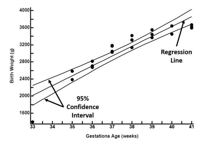
Example: We wish to know if gestational age (in weeks) and birth weight (in grams) are correlated. We obtained the data as shown in the first 2 columns of the table to the right, where X Val is gestational age in weeks, and Y Val is birth weight in grams.
Pearson's Correlation analysis obtained the following results
Correlation Coefficient ρ = 0.9237, Standard Error=0.0857
Assuming ρ to be normally distributed, p=<0.0001(two tails) and p=<0.0001(one tail). As the 1 tail p<0.05, we can conclude a significant correlation exists
Using Fisher's Z for calculation, the 95% confidence interval for ρ are
1 tail = >0.8447, or <0.9633
2 tail = 0.8223 to 0.9682
As the lower limit of the 1 tail CI exceeds the null value of 0, we can conclude that significant correlation exists
Linear Regression
Linear regression describes the relationship between an independent variable (x) and a dependent variable (y). The relationship is directional in that x comes before y, and x values predicts or influences the values of y.
The values of y are assumed to be continuous and normally distributed while x can be binary, ordinal, or continuous measurements that are not necessarily normally distributed
The regression formula is y = a + bx, where a is the constant, the value of y when x=0, and b is the regression coefficient, the change in y value for each unit of change in x value.
The regressed value of y is the mean value for y given x. Its error is a combination of the Standard Error of b and the Standard Error of mean y. Because of this combination, the error of regressed y changes with the value of x, less near the mean and widens towards the extremes.
Example: Using the same example as the for correlation, the results of calculations are
The sample size is 22
mean x = 37.8, sum of square x = 95.86
The regression equation is birth weight in gram (y) = -5584.9 + 230.3(gestational age in weeks (x))
The Standard Error of the regression coefficient SEb = 21.4
The residual variance after regression = 43747.59
The Standard error of y from regression value (SEYx) depends on the x value and
= sqrt(residual means squares(1/n + (x-meanx)2/sum squares x))
= sqrt(43747.59(1 / 22 + (x -37.8)2 / 95.86))
95% CI of y for any x value
= yx ± t(for 95%CI) * SEYx)
= -5584.8 + 230.3x ± 2.086(sqrt(43747.59(1 / 22 + (x - 37.8))))
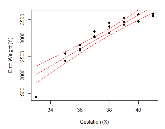
Using these equations, the regressed value of y (RegY), its 95% confidence interval, and the departure of each y value from this regressed mean can be calculated, and presented in the appropriate columns in the table above and to the right. The input data, the regression line, and the 95% confidence interval can also be plotted as shown to the right
References
Correlation and Regression Analysis
Armitage P (1980) Statistical Methods in Medical Research. Blackwell Scientific
Publications, Oxford UK. ISBN 0-632-05430-1 p. 147-166.
Significance and 95% confidence interval of correlation coefficient
t test : Armitage P. Statistical Methods in Medical Research (1971).
Blackwell Scientific Publications. Oxford. P.156-163.
Confidence Interval : Altman DG, Machin D, Bryant TN and Gardner MJ. (2000)
Statistics with Confidence Second Edition. BMJ Books ISBN 0 7279 1375 1. p. 89-92
Data Entry: Data is in 2 columns
- Each row representing data from a subject
- Column 1 being the independent x variable
- Column 2 being the dependent y variable
MacroPlot Code
R Code
The following is a single R program, but divided into parts so it is easier to follow
# Correlation
n = nrow(df)
meanX = mean(df$X)
sdX = sd(df$X)
meanY = mean(df$Y)
sdY = sd(df$Y)

# Initial output of parameters
n                     # sample size
c(meanX, sdX)         # mean and SD x
c(meanY, sdY)         # mean and SD Y
cor.test(df$X,df$Y)   # Correlation results
The results are as follows
> # Initial output of parameters
> n                     # sample size
[1] 22
> c(meanX, sdX)         # mean and SD x
[1] 37.772727  2.136571
> c(meanY, sdY)         # mean and SD Y
[1] 3113.955  532.697
> cor.test(df$X,df$Y)   # Correlation results as output by R

	Pearson's product-moment correlation

data:  df$X and df$Y
t = 10.78, df = 20, p-value = 8.814e-10
alternative hypothesis: true correlation is not equal to 0
95 percent confidence interval:
 0.8222882 0.9682270
sample estimates:
     cor
0.923674
Part 3: Regression Analysis
# regression
regRes <- lm(df$Y ~ df$X)
mxC <- summary(regRes)$coefficients
a = mxC[1,1]                              # constant
b = mxC[2,1]                              # regression
ssx = sdX^2 * (n - 1)                     # sum square x
ssy = sdY^2 * (n - 1)                     # sum square y
sxy = b * ssx                             # sum product
rv = (ssy - sxy**2 / ssx) / (n - 2);      # Residual mean Squares
seB = sqrt(rv / ssx);                     # SE of slope b
tB = b / seB                              # t
p = (1 - pt(abs(b), n-2)) * 2             # Type I error 2 tail
t95 = abs(qt(0.025,n-2))                  # t value for p=0.05 2 tail
ll = b - t95 * seB                        # lower limit 95% CI b
ul = b + t95 * seB                        # upper limit 95% CI b
# output regression analysis
regRes          # Regression results as output by R
c(a,b,seB,tB,p) # result of regression a, b, SE, t and p
c(ll,ul)        # 95% CI regression coefficient b
The results are as follows
> # output regression analysis
> regRes          # Regression results as output by R

Call:
lm(formula = df$Y ~ df$X)

Coefficients:
(Intercept)         df$X
    -5584.9        230.3

> c(a,b,seB,tB,p) # result of regression a, b, SE, t and p
[1] -5584.85917   230.29350    21.36240    10.78032     0.00000
> c(ll,ul)        # 95% CI regression coefficient b
[1] 185.7323 274.8547
Part 4: Add regressed values to the data frame
# create regressed values
df$Regy <- a + b * df$X                                   # regressed y value
df$SE_RY <- sqrt(rv * (1 / n + (df$X - meanX)^2 / ssx))   # SE
df$CI_low <- df$Regy - t95 * df$SE_RY                     # 95% CI low
df$CI_high <- df$Regy + t95 * df$SE_RY                    # 95% CI high
df$Zy <- (df$Y - df$Regy) / df$SE_RY                      # z of Y related to regressed y
df # display input data and regressed values
# plot
df <- df[order(df$X),]          # sort data frame by order of x
par(pin=c(4.2, 3))              # set plotting window to 4.2x3 inches
plot(x   = df$X,                # x = Gest age on the x axis
     y   = df$Y,                # y BWt on the y axis
     pch = 16,                        # size of dot
     xlab = "Gestation (X)",       # x label
     ylab = "Birth Weight (Y)")     # y lable
lines(df$X, df$Regy, col = "red")              # regression line
lines(df$X, df$CI_low, col = "red")                # low value 95% CI regression line
lines(df$X, df$CI_high, col = "red")              # high value 95% CI regression line