Macroplot plotting is controlled by the macros in the text area provided.
Each macro must occupy its own line. If the first character of a macro is not A-Z, the line will be considered a comment and ignored
The first macro, which is obligatory, initializes the plot. The macro is
Bitmap Initialize width(in pixels), height(in pixels), red(0-255) blue(0-255), green(0-255) transparency(0-255)
Example : Bitmap Initialize 700 500 255 255 255 255 which provides a landscape area 700 pixels wide, 500 pixel high, with white background
The following are default settings when the bitmap is initiated.
Lines are black (0 0 0 255) and 3 pixels in width
Fill color for bars and dots are black (0 0 0 255), and the fill type is set to fill only (1) (see Fill Type)
Dots (circl and square) are set to 5 pixels radius (diameter=11 pixels)
Fonts are set as follows
Font face is set to sans-serif. Serif, sans-serif, and monospace are available to all browsers, user can use any font available to his/her browser
Font size is set to 16 pixels high
Font color, both line and fill are set to black (0 0 0 255), and fill type to 1 (fill only) (see Font Type)
Macros for plotting on the bitmap begin with the keyword Bitmap, and the coordinates are x=number of pixels from the left border and y=number of pixels from the top border
A central plotting area is also defined
By default, at initialization, as 15% from the left and bottom, 5% from right and top
defined by user as Plot Pixels left top right bottom, these being number of pixels from the left and top border
e.g. Plot Pixels 105 25 665 425 would be the same as the default setting for a bitmap of 700 pixels wide and 500 pixels high
The values of the data used in plotting in this central area can be defined as follows
Plot Values left top right bottom, these being the extreme values used in the data
e.g.Plot Values 0 100 10 50 represents x values of 0 on the left to 10 to the right, and y values of 50 at the bottom to 100 to the top
After the values are declared, all plotting in the central area uses macros beginning with the keyword Plot, and the coordinates are the values in the data
Macros
This panel lists and describes all macros used in this version of MacroPlot by Javascript. They are divided into the following sub-panels
Initialization and settings
Plotting areas, coordinates used, and drawing of x and y axis
Drawing lines, bars, dots, text, and other shapes
Initialization
This sub-panel lists those macros that initialized the bitmap, and set the parametrs for drawing
Initialize Plotting
Bitmap Initialize w h r g b t is the first and obligatory macro, which Initializes the bitmap
w and h are width and height of the bitmap in number of pixels. The most common dimensions are
w=700 and h= 500 for landscape orientation
w=500 and h=700 for portrait orientation
Both 500 for square bitmap
r g b t represents red, green, blue and transparency values for the background, each value is 0 for non-existence to 255 for maximum intensity. The most commonly used background is white (255 255 255 255)
For most plotting programs in StatsToDo the macro used is Bitmap Initialize 700 500 255 255 255 255, a landscape orientation with white background
Settings for lines
The settings provide parameters for all subsequent plotting until the parameter is reset
Line Color r g b t sets the line color of red, green, blue and transparency values, each value is 0 for non-existence to 255 for maximum intensity. On initialization of the bitmap, line color is lines is set by default to black (0 0 0 255)
Line Thick p sets the thickness of lines to p pixels. On initialiszation, the default setting is 3 pixels for line thickness
Settings for fills
When bars, dots, arcs and wedges are plotted, the interior of these symbols are called fills, and they are set as follows
Fill Color r g b t sets the filling color of red, green, blue and transparency values, each value is 0 for non-existence to 255 for maximum intensity. On initialization of the bitmap, fill color is lines is set by default to black (0 0 0 255).
Fill Type t sets how the fills are to be used, t can be one of the following
t=0: only the outline, defined by the line parameters, are plotted. Fill is ignored
t=1: only fill is carried out, outline is ignored
t=2: both outline and fill are plotted
When the plot is initialized, the default setting for fill type is t=1
Settings for fonts
These set the font characteristics for text output. Please note: settings for lines and fills for fonts are separate and independent to those for general line and shape plottings
Font Face name sets the font face. The program will accept all fonts supported by the user's border. The 3 fonts accepted by all browsers are serif, sans-serif, and monospace. On initialization, sans-serif is set by default
Font Style s where s can be either normal or bold. On initialization the default setting is bold
Font Size h where h is the height of the text in pixels. On initialization, the default font size is set to 16
Font Thick p where p is the thickness of the outline of the font. On initialization, this is set to p=1
Font LColor r g b t sets the color of the outline of the font. On initialization this is set to black (0 0 0 255)
Font FColor r g b t sets the fill color of the of the font. On initialization this is set to black (0 0 0 255)
Font Color r g b t sets both LColor and FColor to the same color. On initialization this is set to black (0 0 0 255)
Font Type t where t determines which part of the font is drawn, and can be one of the following
t=0: only the outline of the font, defined by the thick and LColor parameter is drawn
t=1: only the fill of the font is drawn
t=2: both outline and fill are drawn
When the plot is initialized, the default setting for Font type is t=1
Please Note: When the bitmap is initialized, the default settings, which are suitable for most situations, are automatically set, so users need not worry about these settings unless he/she has a different preference.
Axis & Coordinates
This sub-panel presents macros that define the plotting areas, and creating the x and y axis for plotting
Drawing on the bitmap
When plotting on the initialized bitmap
the horizontal coordinate x is the number of pixels from the left border
the vertical coordinate y is the number of pixels from the top border
The macro used begins with the keyword Bitmap
Drawing on the plotting area
In most cases, there is a need to draw and label the x and y axis, and drawing coordinates used are the actual values of the data. The macros used for these all begins with the keyword Plot, and are purposes are as follows
Plot Pixels lp tp rp bp defines an area for plotting
lp defines the left border of the plotting area, in the number of pixels from the left border of the bitmap. In most cases this is 15% of the bitmap's width
tp defines the top of the plotting area, in the number of pixels from the top border of the bitmap. In most cases this is 5% of the height
rp defines the right border of the plotting area, in the number of pixels from the left border of the bitmap. In most cases this is 95% of the width (or 5% from the right border of the bitmap)
bp defines the bottom border of the plotting area, in the number of pixels from the top border of the bitmap. In most cases this is 85% of the height (or 15% from the bottom)
An example is that is that, in a landscape orientated bitmap of 700 pixels width and 500 pixel height, Plot Pixels 105 25 665 425 sets the central area for plotting that is 15% from the left and bottom, and 5% from the top and right.
This macro is usually not necessary if the 5%/15% setting suits the user, as this is the default setting when the bitmap is initialized
Plot Values lv tv rv bv defines the data values to be used in plotting
lv is the extreme data value for the horizontal variable x on the left
tv is the extreme data value for the vertical variable y at the top
rv is the extreme data value for horizontal variable x on the right
bv is the extreme data value for the vertical variable y at the bottom
Plot Logx 1 sets the horizontal x axis to the log scale. Normal scale is set on initialization, or reset by Plot Logx 0
Plot Logy 1 sets the vertical y axis to the log scale. Normal scale is set on initialization, or reset by Plot Logy 0
Plot XLabel label distance places the label for the horizontal x axis, below the bottom of the plotting area
lable is a single word text string, using the underscore _ to represent spaces if necessary
space is the number of pixels between the bottom of the plot area and the label text string
Plot YLabel label distance places the label for the vertical y axis, on the left of plotting area
lable is a single word text string, using the underscore _ to represent spaces if necessary
space is the number of pixels between the left of the plot area and the label text string
The quickest and easiest way to draw axis
The following 4 macros are sufficient to draw the x and y axis under most circumstances
Plot XAxis y nsIntv nbIntv len gap line will mark out and numerate the horizontal x axis
y is the y value on which the x axis lie
nsIntv is the number of small intervals between the vertical line marks, 10 to 20 are recommended
nbIntv is the number of big intervals between the numerical scales, 5 to 10 are recommended
len is the length of the mark in pixels, +ve value downwards and negative value upwards. -10 is recommended
gap is the number of pixels between the numerical scaling text and the y value of the axis, +ve values for text below axis and negative value for text above axis. 3 is recommended
Line determines the axis line is drawn, 0 for no line, 1 for line
Plot YAxis x nsIntv nbIntv len gap line will mark out and numerate the vertical y axis
x is the x value on which the y axis lie
nsIntv is the number of small intervals between the horizontal line marks, 10 to 20 are recommended
nbIntv is the number of big intervals between the numerical scales, 5 to 10 are recommended
len is the length of the mark in pixels, +ve value to the right and negative value to the left. 10 is recommended
gap is the number of pixels between the numerical scaling text and the y value of the axis, +ve values for text to the right of axis and negative value for text to the left of axis. -3 is recommended
Line determines the axis line is drawn, 0 for no line, 1 for line
Plot AutoXLogScale y len gap line will mark and numerate the x axis if it is in log scale
The x axis must be set to the log scale by Plot Logx 1. If axis not set to log this macro will abort
y is the y value on which the x axis lie
len is the length of the mark in pixels, +ve value downwards and negative value upwards. -10 is recommended
gap is the number of pixels between the numerical scaling text and the y value of the axis, +ve values for text below axis and negative value for text above axis. 3 is recommended
Line determines the axis line is drawn, 0 for no line, 1 for line
Plot AutoYLogScale x len gap line will mark and numerate the y axis if it is in log scale
The y axis must be set to the log scale by Plot Logy 1. If axis not set to log this macro will abort
x is the x value on which the x axis lie
len is the length of the mark in pixels, +ve value downwards and negative value upwards. -10 is recommended
gap is the number of pixels between the numerical scaling text and the y value of the axis, +ve values for text below axis and negative value for text above axis. 3 is recommended
Line determines the axis line is drawn, 0 for no line, 1 for line
Other methods of drawing axis
Users may wish to draw individual part of the axis, and the following macros can be used
Plot XLine y Draws the horizontal x axis line at the y value y
Plot YLine x Draws the vertical y axis line at the x value y
Plot XMark y begin interval len marks the horizontal x axis with a series of vertical marks
y is the y value where the axis is to be marked
begin is the value for the first mark
interval is the interval between marks
len is the length of the mark line in pixels, +ve downwards, -ve upwards
Plot YMark x start interval len marks the vertical y axis with a series of horizontal marks
x is the x value where the axis is to be marked
start is the value for the first mark
interval is the interval between marks
len is the length of the mark line in pixels, +ve to the right, -ve to the left
Plot XScale y start interval gap writes the numerical scales for the horizontal x axis
y is the y value for the axis
start is the first value to be written
interval is the interval between numerical scales
gap is the space in pixels between the scale text and the axis, +ve for text below axis, -ve for text above axis
The number of decimal points in the scale is the same as that of the interval value
Plot YScale x start interval gap writes the numerical scales for the vertical y axis
x is the x value for the axis
start is the first value to be written
interval is the interval between numerical scales
gap is the space in pixels between the scale text and the axis, +ve for text to the right of axis, -ve for text to the left of axis
The number of decimal points in the scale is the same as that of the interval value
Plot XMarkIntv y interval len marks the horizontal x axis with a series of vertical marks
y is the y value of the axis
interval is the interval between the marks, beginning at 0 and while in range
len is the length of the mark line in pixels, +ve downwards, -ve upwards
Plot YMarkIntv x interval len marks the vertical y axis with a series of horizontal marks
x is the x value of the axis
interval is the interval between the marks, beginning at 0 and while in range
len is the length of the mark line in pixels, +ve to the right, -ve to the left
Plot XScaleIntv y interval gap writes the numerical scales for the horizontal x axis
y is the y value of the axis
interval is the interval between the numerical scales, beginning at 0 and while in range
gap is the space in pixels between the scale text and the axis, +ve for text below axis, -ve for text above axis
The number of decimal points in the scale is the same as that of the interval value
Plot YScaleIntv x interval gap writes the numerical scales for the vertical y axis
x is the x value of the axis
interval is the interval between the numerical scales, beginning at 0 and while in range
gap is the space in pixels between the scale text and the axis, +ve for text to the right of axis, -ve for text to the left of axis
The number of decimal points in the scale is the same as that of the interval value
Drawings
This sub-panel describes those macros that draws the plotting objects. Drawing are performed in two environments
Macros that begins with the keyword Bitmap uses pixel values as coordinates, where x is the number of pixels from the left border, and y the number of pixels from the top border
Macros that begins with the keyword Plot uses actual data values (as defined in the Plot Values lv tv rv bv macro, as coordinates
Drawing lines
The thickness and color of any line drawn is set by the Line macros (see setting sub-panel). The default setting is black line 3 pixels in width
Bitmap Line x1 y1 x2 y2 draws the line from x1y1 to x2y2
x1 and x2 are number of pixels from the left border
y1 and y2 are number of pixels from the top border
Plot Line x1 y1 x2 y2 draws the line from x1y1 to x2y2
x1 and x2 are data values for the horizontal variable x
y1 and y2 are data variables for the vertical variable y
Plot PixLine x y hpix vpix draws a line
x and y are data values for the horizonal x value and verticsl y value. This defines the coordinate at the origin of the line
hpix is the number of pixels horizontally from the origin, +ve value to the right, -ve value to the left
vpix is the number of pixels vertically from the origin, +ve value downwards, -ve value upwards
The line is then drawn between the origin and that defined by hpix and vpix
Drawing bars
The color and thickness of the outline are defined in the Line macro. The color of the fill is defined in the fill color and Fill Type macro. The default setting is black (0 0 0 255) for both line and fill color, and the Fill type is set to 1, only the fill and no outlines. These settings are suitable for most circumstances, but user can change them is so required.
Bitmap Bar x1 y1 x2 y2 draws a bar the corner of which are x1y1 and x2y2. X and y are number of pixels from the left and top border of the bitmap
Plot Bar x1 y1 x2 y2 draws a bar the corner of which are x1y1 and x2y2. X and y are data values as defined in Plot Values lv tv rv bv
Bar Wide w sets the width / height of bars for Plot VBar and Plot HBar
w is the half width of the bar, so a VBar is 2w+1 pixels in width, and HBar is 2w+1 pixels in height
The default value for w is 7 pixels (making width/height of 15 pixels), unless the user changes it
Plot VBar x y1 y2 hshift draws a vertical bar
x is the data value for the horizontal x variable. The is the center of the vertical bar
y1 and y2 are values for the vertical y variable. They define the vertical ends of the bar
hshift is the number of pixels the whole bar is shefted horizontally, +ve value to the left and +ve value to the right. In most cases this is 0 (no shift). However, if there are more than 1 bar in the same position, shifting some of them will avoid the bars overlapping and obscuring each other
The width of the vertical bar is set by default at 7, (width of bar=15 pixels)
Plot HBar x1 x2 y vshift draws a horizontal bar
x1 and x2 are data values for the horizontal x variable. They define the horizontal ends of the bar
y is the value for the vertical y variable, and defines and center of the horizontal bar
vshift is the number of pixels the whole bar is shefted vertically, -ve value upwards and +ve value downwards. In most cases this is 0 (no shift). However, if there are more than 1 bar in the same position, shifting some of them will avoid the bars overlapping and obscuring each other
Theheight of the horizontal bar is set by default at 7, (height of bar=15 pixels)
Drawing dots
There are only 2 dot types, circle and square. If more than 2 tyoes of dats are required, they can be distinguished by the colours of the outline and fill, and by their sizes. Settingsd for dot parameters are in the settings sub-panel
Bitmap Circle x y radius and Bitmap Square x y radius draws a circle or a square dot
x and y are the number of pixels from the left and top border
Radius is in number of pixels. The diameter of the dot is 2Radius+1 pixels
Plot Circle x y radius hshift vshift and Plot Square x y radius hshift vshift draws a circle or a square dot
x and y are the data values of the horizontal x variable and vertical y variable, as defined by Plot Values lv tv rv bv
Radius is in number of pixels. The diameter of the dot is 2Radius+1 pixels
hshift is the number of pixels the dot is shifted horizontally, -ve value to the left, +ve value to the right
vshift is the number of pixels the dot is shifted vertically, -ve value upwards, +ve value downwards
In most cases there is no shift (0 0), but id there are more than 1 dot in the same position, shifting avoids the dots superimposing over and obscuring each other
Dot Radius r sets the radius of the dot in pixels. The diameter of the dot is 2radius+1 pixels. The default radius is 5
Dot Type t where t is either circle or square. The default setting is circle
Plot Dot x y hshift vshift draws the dot, with its parameters (shape size color outline fill) already pre-set
x and y are the data values of the horizontal x variable and vertical y variable, as defined by Plot Values lv tv rv bv
hshift is the number of pixels the dot is shifted horizontally, -ve value to the left, +ve value to the right
vshift is the number of pixels the dot is shifted vertically, -ve value upwards, +ve value downwards
In most cases there is no shift (0 0), but if there are more than 1 dot in the same position, shifting avoids the dots superimposing over and obscuring each other
Drawing text
The color, outline, fill, font, and weight of text are preset (see settings). The default settinfs are sans-sherif, black fill only, and 16pxs high
Bitmap HText x y ha va txt draws text horizontally on the bitmap
x and y are number of pixels fom the left and top borders, and together being the reference coordinate of the text
ha is horizontal adjust
ha=0: the left end of the text is at the x coordinate
ha=1: the center of the text is at the x coordinate
ha=2: the right end of the text is at the x coordinate
va is vertical adjust
va=0: the top of the text is at the y coordinate
va=1: the center of the text is at the x coordinate
va=2: the bottom end of the text is at the x coordinate
txt is the text to be drawn. It must be a single word with no gaps. Spaces can be represented by the underscore _
Plot HText x y ha va txt hshift vshift draws text horizontally on the bitmap
x and y are data values as defined by Plot Values lv tv rv bv, and together being the reference coordinate of the text
ha is horizontal adjust
ha=0: the left end of the text is at the x coordinate
ha=1: the center of the text is at the x coordinate
ha=2: the right end of the text is at the x coordinate
va is vertical adjust
va=0: the top of the text is at the y coordinate
va=1: the center of the text is at the x coordinate
va=2: the bottom end of the text is at the x coordinate
txt is the text to be drawn. It must be a single word with no gaps. Spaces can be represented by the underscore _
hshift is the number of pixels the text is shifted horizontally, -ve value to the left, +ve value to the right
vshift is the number of pixels the text is shifted vertically, -ve value upwards, +ve value downwards
In most cases there is no shift (0 0), but if there are other structures in the same position, shifting avoids the text and structures obscuring each other
Bitmap VText x y ha va txt draws text vertically (90 degrees anticlockwise from horizontal) on the bitmap
x and y are number of pixels fom the left and top borders, and together being the reference coordinate of the text
ha is horizontal adjust
ha=0: the left end of the text is at the x coordinate
ha=1: the center of the text is at the x coordinate
ha=2: the right end of the text is at the x coordinate
va is vertical adjust
va=0: the top of the text is at the y coordinate
va=1: the center of the text is at the x coordinate
va=2: the bottom end of the text is at the x coordinate
txt is the text to be drawn. It must be a single word with no gaps. Spaces can be represented by the underscore _
Plot VText x y ha va txt hshift vshift draws text vertically (90 degrees anticlockwise from horizontal) on the bitmap
x and y are data values as defined by Plot Values lv tv rv bv, and together being the reference coordinate of the text
ha is horizontal adjust
ha=0: the left end of the text is at the x coordinate
ha=1: the center of the text is at the x coordinate
ha=2: the right end of the text is at the x coordinate
va is vertical adjust
va=0: the top of the text is at the y coordinate
va=1: the center of the text is at the x coordinate
va=2: the bottom end of the text is at the x coordinate
txt is the text to be drawn. It must be a single word with no gaps. Spaces can be represented by the underscore _
hshift is the number of pixels the text is shifted horizontally, -ve value to the left, +ve value to the right
vshift is the number of pixels the text is shifted vertically, -ve value upwards, +ve value downwards
In most cases there is no shift (0 0), but if there are other structures in the same position, shifting avoids the text and structures obscuring each other
Other miscellaneous drawings
Bitmap Arc x y radius startDeg endDeg rotate draws an arc.
x and y are number of pixels from the left and top border, and together form the center of the arc
radius is the radius of the arc, in number of pixels
startDeg and endDeg are the degrees (360 degrees in full circle) of the arc
rotate defines the direction of the arc, 0 for clockwise, 1 for anti-clockwise
Bitmap Wedge x y radius startDeg endDeg shift rotate draws a wedge, essentially an arc with lines to the center
x and y are number of pixels from the left and top border, and together form the center of the wedge
radius is the radius of the edge, in number of pixels
startDeg and endDeg are the degrees (360 degrees in full circle) of the wedge
shift is the number of pixels that the wedge is moved centrifugally (away from the center). This is used in pie charts to separate the wedges of the pie
rotate defines the direction of the wedge, 0 for clockwise, 1 for anti-clockwise
Plot Curve a b1 b2 b3 b4 b5 x1 x2 draws a polynomial curve
The curve is y=a + b1x + b2x2 + b3x3 + b4x4 + b5x5. Where higher power is not needed, 0 is used to represent the the coefficient b
The curve is drawn from data value x from x1 to x2
Plot Normal mean sd height draws a normal distribution curve
mean and sd (Standard Deviation) are as in the data horizontal variable variable x
height is the maximum height (where x=mean) of the curve as in the vertical variable y
Color Palettes
Plain Colors
0 0 0 #000000
0 0 63 #00003f
0 0 127 #00007f
0 0 191 #0000bf
0 0 255 #0000ff
0 63 0 #003f00
0 63 63 #003f3f
0 63 127 #003f7f
0 63 191 #003fbf
0 63 255 #003fff
0 127 0 #007f00
0 127 63 #007f3f
0 127 127 #007f7f
0 127 191 #007fbf
0 127 255 #007fff
0 191 0 #00bf00
0 191 63 #00bf3f
0 191 127 #00bf7f
0 191 191 #00bfbf
0 191 255 #00bfff
0 255 0 #00ff00
0 255 63 #00ff3f
0 255 127 #00ff7f
0 255 191 #00ffbf
0 255 255 #00ffff
63 0 0 #3f0000
63 0 63 #3f003f
63 0 127 #3f007f
63 0 191 #3f00bf
63 0 255 #3f00ff
63 63 0 #3f3f00
63 63 63 #3f3f3f
63 63 127 #3f3f7f
63 63 191 #3f3fbf
63 63 255 #3f3fff
63 127 0 #3f7f00
63 127 63 #3f7f3f
63 127 127 #3f7f7f
63 127 191 #3f7fbf
63 127 255 #3f7fff
63 191 0 #3fbf00
63 191 63 #3fbf3f
63 191 127 #3fbf7f
63 191 191 #3fbfbf
63 191 255 #3fbfff
63 255 0 #3fff00
63 255 63 #3fff3f
63 255 127 #3fff7f
63 255 191 #3fffbf
63 255 255 #3fffff
127 0 0 #7f0000
127 0 63 #7f003f
127 0 127 #7f007f
127 0 191 #7f00bf
127 0 255 #7f00ff
127 63 0 #7f3f00
127 63 63 #7f3f3f
127 63 127 #7f3f7f
127 63 191 #7f3fbf
127 63 255 #7f3fff
127 127 0 #7f7f00
127 127 63 #7f7f3f
127 127 127 #7f7f7f
127 127 191 #7f7fbf
127 127 255 #7f7fff
127 191 0 #7fbf00
127 191 63 #7fbf3f
127 191 127 #7fbf7f
127 191 191 #7fbfbf
127 191 255 #7fbfff
127 255 0 #7fff00
127 255 63 #7fff3f
127 255 127 #7fff7f
127 255 191 #7fffbf
127 255 255 #7fffff
191 0 0 #bf0000
191 0 63 #bf003f
191 0 127 #bf007f
191 0 191 #bf00bf
191 0 255 #bf00ff
191 63 0 #bf3f00
191 63 63 #bf3f3f
191 63 127 #bf3f7f
191 63 191 #bf3fbf
191 63 255 #bf3fff
191 127 0 #bf7f00
191 127 63 #bf7f3f
191 127 127 #bf7f7f
191 127 191 #bf7fbf
191 127 255 #bf7fff
191 191 0 #bfbf00
191 191 63 #bfbf3f
191 191 127 #bfbf7f
191 191 191 #bfbfbf
191 191 255 #bfbfff
191 255 0 #bfff00
191 255 63 #bfff3f
191 255 127 #bfff7f
191 255 191 #bfffbf
191 255 255 #bfffff
255 0 0 #ff0000
255 0 63 #ff003f
255 0 127 #ff007f
255 0 191 #ff00bf
255 0 255 #ff00ff
255 63 0 #ff3f00
255 63 63 #ff3f3f
255 63 127 #ff3f7f
255 63 191 #ff3fbf
255 63 255 #ff3fff
255 127 0 #ff7f00
255 127 63 #ff7f3f
255 127 127 #ff7f7f
255 127 191 #ff7fbf
255 127 255 #ff7fff
255 191 0 #ffbf00
255 191 63 #ffbf3f
255 191 127 #ffbf7f
255 191 191 #ffbfbf
255 191 255 #ffbfff
255 255 0 #ffff00
255 255 63 #ffff3f
255 255 127 #ffff7f
255 255 191 #ffffbf
255 255 255 #ffffff
Color Palletes
Table of colors used on this web site
255 255 255 #ffffff
224 224 224 #e0e0e0
128 128 128 #808080
128 0 0 #800000
255 0 0 #ff0000
96 48 96 #603060
48 16 64 #301040
96 96 160 #6060a0
160 160 96 #a0a060
160 160 0 #a0a000
153 191 164 #99bfa4
160 160 96 #a0a060
97 24 0 #611800
204 63 200 #cc3fc8
224 224 224 #e0e0e0
Patterns of complementary colors
A
105 93 70 #695d46
255 113 44 #ff712c
207 194 145 #cfc291
161 232 217 #a1e8d9
255 246 197 #fff6c5
B
115 0 70 #730046
201 60 0 #c93c00
232 136 1 #e88801
255 194 0 #ffc200
191 187 17 #bfbb11
C
97 24 0 #611800
140 115 39 #8c7327
71 164 41 #47a429
153 191 164 #99bfa4
242 239 189 #f2efbd
D
20 87 110 #14576e
140 33 90 #8c215a
230 133 38 #e68526
195 102 163 #c366a3
242 207 242 #f2cff2
E
64 1 1 #400101
48 115 103 #307367
96 166 133 #60a685
242 236 145 #f2ec91
229 249 186 #e5f9ba
F
55 89 21 #375915
166 60 60 #a63c3c
115 108 73 #736c49
166 157 129 #a69d81
242 224 201 #f2e0c9
G
115 36 94 #73245e
166 69 33 #a64521
217 182 78 #d9b64e
242 218 145 #f2da91
242 242 242 #f2f2f2
H
255 77 0 #ff4d00
102 87 71 #665747
125 179 0 #7db300
153 138 122 #998a7a
217 195 98 #d9c362
I
128 0 38 #800026
128 128 83 #808053
92 153 122 #5c997a
163 204 143 #a3cc8f
255 230 153 #ffe699
Explanations
This page provides explanations, clarifications, and supports to Linear Discriminant Analysis, as shown in the Javascript program, and the R codes
Discriminant Analysis is clearly and succinctly described in Wikipedia, and only a brief description will be provided here, to help the user to understand the data input required and interpreting the results.
Different approaches to calculations
Discriminant Analysis was introduced by Fisher more than a century ago, as a variant of the multiple regression model, but with multinomial groups as dependent variable and normally distributed measurements as independent variable. It enjoys continued usage, but with time many modifications and additions are made, producing options for users to produce results that are conceptually similar but numerically different. This confusion is further aggravated by some statistical packages keeping to the original algorithm, some including useful additions and and modifications, and some providing menus from which users can choose different options. The following comments attempts to clarify some of these issues
The original algorithm used actual measurements of independent variables and their covariate matrix for Principal Component extraction. The problem is that the results can be distorted if the scalars of different variables differ widely. For example, using height in inches and weight in pounds will produce numerically different results from the same data using cms and Kgs. Increasingly therefore the original measurements are normalized to Standard Deviation units z, where z=(value-mean)/SD, so that all independent variables are converted to have a mean of 0 and Standard Deviation of 1 before they are used.
Statistical packages vary in how this problem is managed. The algorithm descibed on this page allows actual values in data input, but converts these to z values for calculating Discriminate functions. To enable the calculation of z values therefore requires the means and Standard Deviations estimated using the modelling data.
The number of Linear Discriminant functions created by the original algorithm is one less than the number of outcome groups (nf=ng-1). Traditionally, all functions are used to estimate the probability of belonging to each group for a case (row of data).
However, it can be clearly demonstrated that, because the functions are essentially transforms of Principal Components, the functions extracted earlier have greater discriminating power than the latter ones, as the latter ones contain mostly statistical noise. To ignore the more trivial functions therefore will create only minor distortions to the numerical results, and in most cases not altering how the results are interpreted.
In the Javascript program on this page, the common convention is followed, and all functions are used in estimating group probability during the validation of the data, and copied to templates for future use. However, the statistical significance of each function is estimated using the chi square test, and those functions that are not statistically significant are identified. This allows the user (if he/she so wishes), to use a reduce set of functions (only the statistically significant ones) on future data.
There are two major reasons for using Discriminant analysis. Firstly, to analyse the structure of the data itself, and interpret the results as scientific realities represented by the data. Secondly, to use the data to create a model, and use that model to interpret future and different sets of similar measurements. Both approaches require the allocation of outcome groups, based on the probabilities that are calculated from the Discriminant Functions. How the probabilities are calculated, however, differ according to the purpose of the analysis.
If the purpose is to analysis and interpret the structure of the data, then apriori probabilities are not included, so that the structure of the model is not distorted. This is the method of calculation in program 1, during the validation of the model.
If the purpose is to use the model already developed, to interpret and classify future and additional data, then the accuracy of prediction is a priority, and the inclusion of apriori probabilities is appropriate, as in program 2 of the Javascript program
To demonstrate this difference, we can imagine an analysis relating a set of symptoms to discriminate headache caused by tension or by brain tumor. To study the relationship between symptoms and diagnosis, a data set representative of the clinical scenario (say from medical records) is used, which contains similar number of cases with tension and brain tumor. From this data, the relationship between symptoms and eventual diagnosis can be established (Maxumum Likelihood). When the model is used clinically to make diagnosis, that headache caused by tension is many times more common than that caused be tumours must be taken in consideration, and a more accurate diagnosis requires the inclusion of the apriori probabilities of these two conditions (Bayesean probability).
Statistical packages differ in the inclusion of a priori probabilities. Many includes a priori probabilities as the default, estimated from the sample sizes of the outcome groups in the reference data. Some use Maximum Likelihood as default. Some require users to insert the priori probabilities. All these approaches are correct in the right context, leaving the options with the user.
The programs in the Javascript program allows both approaches. In program 1, when the model is developed, the validation examines the structure of the data, so no apriori probabilities are included. In program 2, when the developed model is used to describe or predict new and additional data, there are provisions for the user to include apriori probabilities
George D and Mallery P (1999) SPSS for Windows Step by Step. A Simple Guide and Reference.
Allyn and Bacon, Sydney. ISBN 0-205-28395-0 Chapter 26. The Discriminant Procedure p.313-328.
Resources used to developed the web bases Javascript program
These are very old books, that still present actual formulae and algortithms for all step in the calculations. Most newer references do not provide detailed algorithms, but advise users to access available packages such as SAS, SPSS, R, and Python
Overall JE and Klett CJ (1972) Applied Multivariate Analysis. McGraw Hill Series in Psychology.
McGraw Hill Book Company New York. Library of Congress No. 73-14716407-047935-6
Chapter 2 p.24-56 : Matrix math. Particularly the Square Root method of matrix inversion.
Also calculations for between and within group Sum Product and Covariance matrices
Chapter 10 p.280-306 : Multiple Discriminant Analysis, particularly the algorithm.
Chapter 13 p. 345-371 Normal Probability Density Model for classification.
Chapter 14 p. 373-383 Use of Canonical Correlates for Classification. Chapters 13 and 14
provided the algorithms for calculating Maximum Likelihood and the Bayesian Probabilities
Press WH, Flannery VP, Teukolsky SA, Vetterling WT (1989). Numerical Recipes in Pascal.
Cambridge University Press IBSN 0-521-37516-9 p.395-396 and p.402-404.
Jacobi method for finding Eigen values and Eigen vectors
Norusis MJ (1979) SPSS Statistical Algorithms Release 8. SPSS Inc Chicago
Chapterr 23 : Discriminant p. 69-83. Formulae for algorithm provided by SPSS.
Useful references and advice on Discriminant analysis using R
Venables, W. N. and Ripley, B. D. (2002) Modern Applied Statistics with S. Fourth edition. Springer.
Javascript Program
Help & Hints
This panel provides supports for data entry and interpretation of results from the Javascript program.
There are two programs.
Program 1 is primary discriminant analysis using a set of modelling data, creating parameters and coefficients that can be used to interpret future new data.
Program 2 is intended for using coefficients and parameters previously established to analyse new sets of data to produce discriminate function values and classify into groups. It provides data inputs for parameters and coefficients previously created, and the new data to be analysed.
on this page, Program 2 is executed automatically as a cascade from program 1, with all the coefficients and parameters established in program 1 copied into the appropriate input for program 2.
Default Example
tannin
color
acidity
sugar
Wine
1.2
45
3.16
72.7
SR
1.3
67
3.38
102.4
SR
1.1
48
3.61
33.7
SR
1.6
36
3.51
58.2
SR
1.5
47
3.20
44.2
DR
1.5
74
3.21
91.8
DR
1.7
47
3.39
53.1
DR
1.6
56
3.36
88.5
DR
1.1
27
3.30
36.3
SW
1.0
53
3.55
74.7
SW
0.9
37
3.23
94.2
SW
1.2
23
3.07
53.8
SW
1.4
44
3.34
20.7
DW
1.3
34
3.24
9.5
DW
1.1
37
3.24
17.8
DW
1.4
55
3.35
35.9
DW
The default example data are artificially created to demonstrate the algorithm, and does not reflect reality. It purports to be a study to discriminate the type of wine (SR for sweet red, DR for dry red, SW for sweet white, and DW for dry white). It uses 4 measurements to do so, col 1 is measurement of tannin, col 2 color, col 3 acidity, and col 4 sugar. Sixteen (16) wines are used to create the model, 4 from each type. The data table is as shown to the right, and entered (without the headers) in the data input text area in the program
Data Entry
The data are entered as a table
All rows must have the same number of columns, each row represents a wine
Each column represents a predictor variable, in this example, in order, tanin, color, acidity, and sugar
The last column on the right is the group labels, and is treated as text. It is a single character or word with no gaps. In this example DR for dry red, DW for dry white, SR for sweet red and SW for sweet white.
Result Output
Groups are organized in alphabetical order, and in this example DR=1, DW=2, SR=3, SW=4
Predictor variables are in the same order as that of the columns in data entry
Discriminate functions are ordered in order of magnitude (statistical significance). The most significant being f1, then f2, f3, etc in decreasing significance. The mark # is used to designate functions that are not statistically significant and can be ignored in subsequent calculations
Step 1: Data Definition
The entered data are summarised. In this example, number of cases (rows) = 16, number of variables = 4 and number of groups = 4.
Table 1a. shows group names in alphabetical order and number of cases in each group
Group 1b shows tha means and Standard Deviations of the variables in the same order as the columns
Step 2: Create Discriminant functions, coefficients and parameters
The values of the predictor variables are converted to z values, where z = (value-mean) / SD, and used in all subsequent calculations. In other words, all values are transformed to have a mean of 0 and SD of 1
An analysis of variance and covariance is carried out to obtained the within group covariance matrix, which is used to produce the Eigen values and vectors in orders of magnitude.
ChiSq
df
p
Func1
92.0895
12
<0.0001
Func2
19.3497
6
0.0036
Func3
1.8596
2
0.3946
Using the eigen values and chi square, the statistical significance of the functions, in decreasing order of chi square and significance is calculated, as shown in the table to the left. Given that there are 4 predictor variables nv=4), the maximum number of functions is nv-1 = 3. However, only the first 2 functions are statistically significant (p<0.05)
Func1
Func2
Func3#
z1
-1.371
0.7463
0.1365
z2
-1.7209
-0.4157
-0.2198
z3
0.6709
0.2961
-0.8886
z4
1.5797
1.4083
0.2128
The Eigen vectors are then used to establish the function coefficients, which are shown in the table to the right. Each function value is the sum of the z value of the variable and the coefficient of the function/variable. Please note that all functional coefficients are presented, the third function is not statistically significant in this example and can be ignored as trivial
Func1
Func2
Func3#
C1
-2.276
1.141
0.279
C2
-1.558
-1.6395
-0.0286
C3
0.6466
0.6087
-0.5464
C4
3.1874
-0.1101
0.2961
Using the function coefficients and the mean z values of each variable in each group, the centroid value of each function (equivlent to the mean) in each group is estimated, as shown in the table to the left. Again values for all 3 functions from this example are calculated, but the third one, being not statistically significant, can be ignored as trivial.
At this point, the initial analysis is completed. The group names, mean and Standard Deviation for rach predictor variables, the function coefficients, and the centroid values, collectively represents the parameters and coefficients of the Discriminant model, and can be used to calculate discriminant functions and allocate to groups any similar data.
Step 3. Validating Analysis
The parameters and coefficients developed are now used to evaluate the modelling data, and check whether the Discriminant calculation predicts the same group as that designated in the modelling data.
Function Scores
Probability of Belonging to Each Group
Grp in Data
Row
Score(f1)
Score(f2)
Score(f3)
DR(1)
DW(2)
SR(3)
SW(4)
1
0.89
0.18
1.05
0.01
0.02
0.81
0.17
SR
2
0.12
1.70
-0.37
0.08
0.00
0.92
0.00
SR
3
1.05
-1.19
-2.07
0.00
0.06
0.89
0.05
SR
4
0.52
1.74
-0.80
0.02
0.00
0.98
0.01
SR
5
-2.47
-0.21
0.75
0.66
0.33
0.00
0.00
DR
6
-3.28
1.27
0.59
0.99
0.00
0.00
0.00
DR
7
-2.28
1.23
-0.23
0.97
0.01
0.01
0.00
DR
8
-1.07
2.28
0.01
0.83
0.00
0.17
0.00
DR
9
2.44
-1.05
0.17
0.00
0.00
0.08
0.92
SW
10
2.94
0.19
-1.55
0.00
0.00
0.19
0.81
SW
11
5.13
0.65
0.74
0.00
0.00
0.00
1.00
SW
12
2.25
-0.23
1.82
0.00
0.00
0.06
0.94
SW
13
-2.13
-1.29
-0.29
0.05
0.94
0.00
0.00
DW
14
-1.34
-2.04
0.35
0.00
0.99
0.00
0.00
DW
15
-0.11
-2.36
0.24
0.00
0.97
0.03
0.00
DW
16
-2.66
-0.87
-0.41
0.20
0.79
0.00
0.00
DW
Each row of the modelling data is analysed in turn. The last column is the designated group, and other columns are the predictor variables. All functions (3 in this example) are used in calculations, although the third function is non-significant and, if ignored, will only make trivial differences to the results
The values of the predictor variables are converted into z values where z = (value - mean) / SD
The function scores are then calculated, each being sum(z x function coefficient) for that function
The distance between the function score and the centroid in each group is then calculated as d = sum(function score - centroid value)2
As d represents Standard Deviations2 from the centroid, the probability of the distance being 0 from a centroid is calculated as exp(-d / 2). This is the probability of belonging to each group
The probabilities in the 4 groups in this example are then normalized to a total of 1 (maximum Likelihood Ratio), and the group with the highest possibility is assuigned as the calculated group.
DR(1)
DW(2)
SR(3)
SW(4)
Total
DR(1)
4
0
0
0
4
DW(2)
0
4
0
0
4
SR(3)
0
0
4
0
4
SW(4)
0
0
0
4
4
Total
4
4
4
4
16
The table showing the results of calculations are shown in the table to the right, and the table counting the comparison between group assigned in the modelling data (row) and as calculated (column) and shown to the left.
The results show that the Discriminate functions correctly assign all the cases. This is not surprising as the data was artificially created to discriminate the groups well. When real data are used, particularly when large number of cases are involved, the random variations involved means that a proportion of erroneous allocation often occurs.
Step 4: Transfer Parameters and Coefficients as Input Data for Program 2
The tables for means and Standard Deviation, the function coefficents, and the centrod values, represents the Discriminant model developed from the modelling data. These are copied to the appropriate text areas of program 2, so they can be used to analyse additional and new data in the future.
Should the user intend to use the coefficients developed in the future, it would be appropriate to archive these parameters and coefficients, so they can be use in future analysis.
Should the user wishes to use only the significant functions, then the last column of the function coefficients and centroid values can be deleted, resulting in the table as follows.
Furthermore, the results can be further altered by Bayesean probability, if the apriori probabilities of the groups are defined.
The results of calculations, using all functions, and having the same apriori probability for all groups, produces the same results as when the data is modelled.
Function Scores
Probability of Belonging to Each Group
Row
Score(f1)
Score(f2)
DR(1)
DW(2)
SR(3)
SW(4)
1
0.89
0.18
0.00
0.01
0.92
0.07
2
0.12
1.70
0.09
0.00
0.90
0.00
3
1.05
-1.19
0.00
0.11
0.68
0.21
4
0.52
1.74
0.03
0.00
0.96
0.01
5
-2.47
-0.21
0.62
0.38
0.01
0.00
6
-3.28
1.27
0.99
0.01
0.00
0.00
7
-2.28
1.23
0.98
0.01
0.01
0.00
8
-1.07
2.28
0.82
0.00
0.18
0.00
9
2.44
-1.05
0.00
0.00
0.10
0.90
10
2.94
0.19
0.00
0.00
0.07
0.93
11
5.13
0.65
0.00
0.00
0.00
1.00
12
2.25
-0.23
0.00
0.00
0.23
0.77
13
-2.13
-1.29
0.06
0.93
0.00
0.00
14
-1.34
-2.04
0.00
0.99
0.00
0.00
15
-0.11
-2.36
0.00
0.97
0.03
0.00
16
-2.66
-0.87
0.23
0.77
0.00
0.00
Step 5: Analyse the Modelling Data
The predictor variables of the reference data are copied to the data input box of program two and analysed. The same table of results as the validating exercise is produced, as shown in the table to the right.
The same input data can be used on clicking the Example button. However this is merely to demonstrate how program 2 can be used. The intention is that users may wish to enter new data here for analysis.
To demonstrate that the third and not significant discriminant function is trivial and unnecessary, the caculations are repeated after the third column from the functions and centroid matrices are deleted, and the results are shown in the table to the right. Comparing to the validating results, the probability coefficients are very similar, and group designations unchanged.
This is essentially a repeat of the validating exercise, and carried out to demonstrate how new data can be analysed.
Step 6
Plotting data
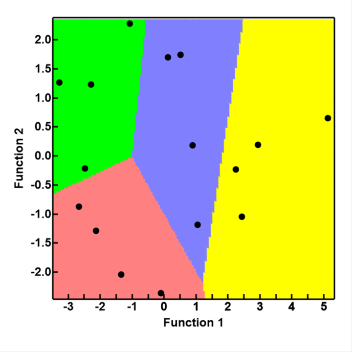
The user can designate any two functions to be plotted in a x/y scatter plot. The program will firstly mark out in color the areas occupied by each group in the plot, then plot the function scores from the two functions in each case as in an x/y scatter plot. The intention is to allow a visual display of the data in any two function, and how they are related to each group.
Ten default background colors are available (assuming that no more than 10 functions will be required in any single Discriminant Analysis). The colors are, in alphabetical order of group names, Grp 1Grp 2Grp 3Grp 4Grp 5Grp 6Grp 7Grp 8Grp 9Grp 10
The plot using the example data with x=function 1 and y=function 2 are as shown above and to the left. The 4 cases from each group can be seen to fit clearly within the areas for each group, with DR (group 1) in green, DW (group 2) in red, SR (group 3) in blue, and SW (group 4) in yellow
It can be seen that function 1 can clearly separate DR (grp 1 green), SR (grp 3 blue) and SW (grp 4 yellow). Data points from DW(grp 2 red) however overaps other groups, and require the additional function 2 to separately identify them
Calculations
Program 1. Produce Discriminant Coefficients from Reference Data
Data Input for Discriminant Analysis Using Reference Data The data is for a single analysis
It is a table of multiple columns
Each row contains data from a case or a record
All columns except the last are predictors and must be numerical
The last column (on the right) is outcome group name, single character or text with no gaps
Program 2. Using Discriminant Coefficients for Calssification
Table of group names Single column of group names in alphabetical order
Table of Means and Standard Deviations of predictor variables Two columns, mean and Standard Deviations
Each row from a predictor variable
Discriminant Fubction Coefficients Number of columns = number of significant functions
Each row from a predictor variable
Function Centroids values Number of columns = number of significant functionss
Each row from a group
Apriori Probabilities Enter apriori probability for each group, separated by spaces
Table of data to be analysed columns are the predictor variables
Each row from a case
x axis
y axis
Functions to plot Enter function numbers for 2D plotting
R Code
The Linear Discriminant analysis using R was carried out to check the accuracy of the Javascript program. Only the minimum amount of coding is used. User can search R for the numerous version of calculation and graphic support for Discriminant analysis.
Please note that R codes are in maroon, and results in blue
Please note: z1, z2, z3, and z4 are the z values for v1, v2, v3, and v4
Step 4. Perform Linear Discriminant analysis and display results
#install.packages("MASS")   # if not already installed
library(MASS)
fit <- lda(Grp ~ z1 + z2 + z3 + z4, data=myDataFrame)
fit
Please note: the calculations are based on the z values and not the original measurements
Prior probabilities of groups:
  DR   DW   SR   SW
0.25 0.25 0.25 0.25

Group means:
            z1         z2         z3         z4
DR  1.14292737  0.7648898 -0.2138289  0.4752644
DW -0.02657971 -0.2303885 -0.1967226 -1.1767538
SR -0.02657971  0.2488196  0.6414866  0.3848597
SW -1.08976796 -0.7833209 -0.2309352  0.3166297

Coefficients of linear discriminants:
          LD1        LD2        LD3
z1  1.3710438 -0.7462890  0.1364612
z2  1.7208986  0.4156835 -0.2198221
z3 -0.6709095 -0.2961205 -0.8885895
z4 -1.5797134 -1.4082862  0.2128178

Proportion of trace:
   LD1    LD2    LD3
0.7899 0.1899 0.0202
The prior probabilities are calculated from the sample sizes of the groups
The LD1, 2, and 3 are the 3 Linear Discriminant functions
The proportion of trace represents the proportion of discriminating power of each function, and can be used to test for statistical significance
Step 5. Calculate function scores
predict(fit,newdata=myDataFrame,prior=c(1,1,1,1)/4)$x #calculate function scores
please note that the prior term is actually unnecesary, as it is not used when function scores are calculated
When the data object is called as newdata, a separate sets of data can be used, providing the the appropriately labelled independent variables are present (in this example z1, z2, z3, and z4)
Please note that the prior term for apriori probability is used here. If this is left out, the program assumes the prior probabilities are the same as that in the reference data, depending on the sample sizes of the groups there.
The function coefficients, scores, and probabilities are the same as that produced by the Javascrip program, other than minor discrepancies caused by different rounding errors.