 | Content Disclaimer Copyright @2020. All Rights Reserved. |
StatsToDo: Probability Explained
Links : Home Index (Subjects) Contact StatsToDo
|
Introduction
This page provides a series of related discussions on probability, the theoretical basis for nearly all the procedures presented on this site.
Probability and Statistics
The scientific approach that characterises the western civilisation is based
on reproducible empirical observations. The idea is that repeatedly observed
relationships or differences are more likely to reflect reality. Another way
of saying this is that, a proposition cannot be accepted unless it is
supported by repeated observations.
Mean, SD, and SE
The problem with repeated observations is that the results, often similar, are not always the same. Experience compels us to abandon the binary idea that something is either true or false. Rather we increasingly see true or false merely as extremes while most of reality is a continuum in between. Similarly, when we consider a scale (e.g. how tall is a man), we can only state an approximation, a range that most would fit in. The uncertainty of reality therefore needs to be approached in a consistent and logical way. Probability is a measurement of how likely things are to occur and is one of the ways to represent uncertainty. Statistics is the set of tools to handle probability.
The ancient Phoenicians were great traders and sea farers, but they tended to overload their boats. In stormy weather, goods had to be thrown overboard in order to save the ship. Owners of lost goods were then compensated by those who did not lose their goods, and the amounts involved depended on the estimated value of the goods. This arrangement was named havara, and this term evolved over the centuries to become average. Statistically the most common and useful expression of average is the mean
Type I Error
The astronomer, Gauss, measured distances between stars. He noticed that it was difficult to reproduce his measurements exactly. However, the measurements clustered around a central value, more common near the mean, and becoming less common as they are further away from the mean. He concluded that any set of measurements would normally distribute to this pattern and called it the Normal Distribution. Following this, De Moivre derived the formula for the Normal Distribution curve in mathematical terms. 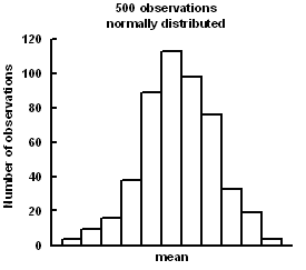 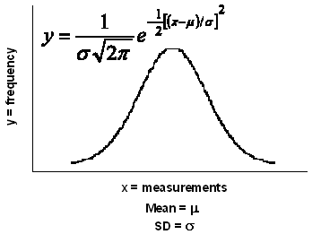
Once this was done, the features of Normal Distribution could be mathematically handled. Using simple calculus, the area under the curve (or any part of it) can be estimated. Fisher developed the concept further and used the area under the curve as a measure of probability. He argued that if the area under the whole curve be consider totality, then any portion represents the probability of the events that describe the portion. From this, he was able to calculate the probability of obtaining a measurement that exceeds a deviation from the mean value. He standardized the measurement of this deviation and called it the Normal Standard Deviate (z), later abbreviated to Standard Deviation, and derived the relationships between z and probability. 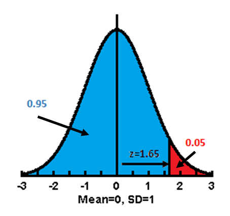
Fisher went on to develop the idea of the Standard Error of the Mean (SE for short). He argued that the true mean is difficult to find, as this requires the measurement of everyone in a population, or an infinite number of times. The mean value obtained in a set of observations is therefore only the sample mean, an estimate of the underlying true mean, and this would vary from samples to samples. An estimate of this variation is called the Standard Error of the Mean (SE). Conceptually, SE represents the Standard Deviation (SD) of the mean values if repeated samples of the same size were taken. In other words, the mean value is calculated for each repeated sample from the population. The SD of these mean values are calculated which equals the SE of the mean.
From the idea of the Standard Error of the mean, Fisher went on to develop the idea of the Standard Error of the Difference. The idea was that, in comparing two groups of observations, the difference between the means of the groups is a sample mean, which also has a Standard Error.
Type II Error
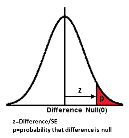
Fisher then derived formulations for the calculation of this Standard Error of the Difference Once these assumptions are accepted, then it follows that the difference between two means is merely the sample mean of a normally distributed measurement. The probability of having a particular value can therefore be calculated. Fisher then ask the question, what is the probability of a particular estimated being different to zero (null). Being a mathematician, Fisher then describe this idea in mathematical terms. In mathematics, one can never prove anything to be true, but one can demonstrate that it is not always true.
Fisher then make the following propositions.
Conceptually the ideas can be simply summarised in the diagram to the right. The development of Probability of Type I Error (α) greatly assisted decision making in agriculture and industry, because it provided a measure of confidence whether an innovation produces better outcome (actually the reverse, the confidence that the innovation makes no difference).
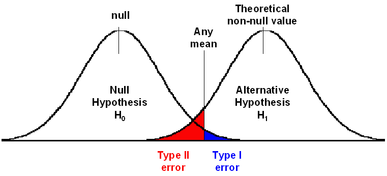
Nearly a generation after Fisher proposed α, Egon Pearson proposed that Type I error was only half the story, and had serious flaws that needed to be addressed. He pointed out a number of problems in using Type I Error (α).
Misuse of Statistical Significance
This error is called the Type II Error, and the probability of its error is call beta (β). Once this schema is set up, α and β can be calculated for any difference (mean) that is observed. The following diagram summarises Pearson's proposals.
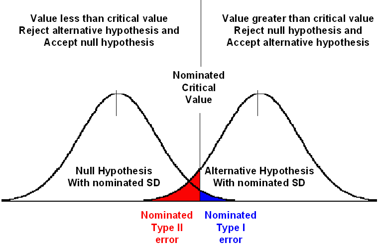
Although Pearson's proposals are conceptually elegant and acceptable, mathematically it was difficult to implement, as the non zero range is infinite. To make the Type II error concept useful, Pearson proposed the following, as shown in the diagram to the right.
The concept of Type II error has frequently been replaced with the term power, where power = 1-β, and this represents the ability to detect a difference if it is really there. Often power is further modified by multiplying it by 100, and presented as a percent. In other words, a β of 0.2 is often presented as a power of 0.8 or 80%.
Statistical significance, as proposed by Pearson, was used extensively for many years, but criticism appeared in the last twenty years of the twentieth century, as increasingly it became noticed that many conclusions drawn using this method were found not to be reproducible.
Recent Developments
The main problem is that the model is highly precise, and the conclusions drawn are only valid if the assumptions made and the procedures carried out complied with the requirements of the model. In practice, this compliance is very difficult. A major difficulty is the correct estimation of the background or within group Standard Deviation at the planning stage, because this value is mostly unknown. Researchers often used published data or conduct pilot studies to obtain this value, but these are sample estimates also, tend to be unstable, and ofen different to that in the data. This problem is compounded when the within group Standard Deviation found in the data differs from that proposed during planning, and the observed SD is used instead of the one proposed during planning. Many researchers seem not to recognise that observed values are sampling values, and are subjected to variations, so they must in most cases differ from the true values. Once the within group Standard Deviation is changed, the sample size initially calculated is no longer valid, and the whole foundation of the model crumbles. A common mistake is to use Pearson's model to calculate sample size, and then to calculate Type I Error(α) using the observations obtained, rejecting or accepting the null hypothesis using the 0.05 criteria. In doing so, the researcher commits the following errors.
Some researchers may even estimate the sample size that could be practically collected, then working backwards to nominate the critical difference or the within group Standard Deviation. In doing so, they present an apparently elegant and legitimate research proposal that can be accepted by regulating bodies, but in reality they have cheated and presented a research model with unrealistic assumptions, so that the results produced are unstable and misleading.
Largely because of errors and misuse, Pearson's model has been increasingly criticised since the 1980s, and research results using this model considered unreliable. The following additional or alternative models have been proposed and are increasingly used.
References
Examining the power
This reference section presents some useful and interesting reading materials
for those interested in understanding statistical probability in greater depth.
Siegel S and Castellan jr. N,J (1988) Nonparametric statistics for the behavioural sciences. McGraw-Hill International Editions Statistics series. ISBN 0-07-057357-3.
Machin D, Campbell M, Fayers, P, Pinol A (1997) Sample Size Tables for Clinical Studies. Second Ed. Blackwell Science IBSN 0-86542-870-0
Cohen J (1988) Statistical power analysis for the behavioral sciences. Second edition. Lawrence Erlbaum Associates, Pubishers. London. ISBN 0-8058-0283-5
Goodman SN (1999) Towards evidence-based medical statistics 1: The p value fallacy. Ann Intern Med. 1999;130: p 995-1004 Goodman SN (1999) Towards evidence-based medical statistics 2: The Bayes Factor. Ann Intern Med. 1999;130: p 1005-1013
|
