This page presents methods for estimating sample size requirements to establish
a proportion. This is frequently needed, to establish the frequencies of events, such as death rates, complication rates, success rates, and so on.
The first approach is to assume that binomial distribution is approximately the same as normal distribution, with the Standard Error depending on the proportion and sample size. From this, the sample size required and the error resulted can be calculated according to the normal distribution model.
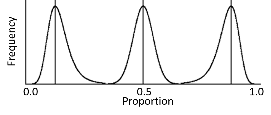
It is also recognised that the binomial distribution is only similar to the normal distribution when the proportion is near 0.5, as the confidence intervals cannot overlap 0 or 1. This means that the distribution becomes increasingly skewed as the proportion becomes increasingly away from 0.5, and this skewness is pronounced when the sample size is small, as shown in the diagram to the left
The second approach is therefore to accept that the binomial distribution is not the same as normal distribution, that it is skewed, narrower towars the ends (0 or 1) and wider towards the middle (0.5). When setting the parameters for calculations, the errors on the two sides of the proportion must be recognised and specified as lower (towards 0) or higher (towards 1).
Terminology
- Confidence is the percent confidence, commonly 80%, 90%, 95%, or 99%
- Proportion (prop) is the proportion
- Error (er) is the error
- When normal distribution is assumed, the confidenc interval is proportion±error
- When binomial distribution is assumed, the confidence interval is from proportion - error(lower side) to proportion + error(higher side)
- Sample size is the sample size required to secure the tolerable error given a proportion
- When normal distribution is assumed, the sample size depends on the symmetrical error
- When binomial distribution is assumed, the sample size differs depending on whether the error refers to the lower or the higher side
Choice of Method
When the proportion is not near end extremes (say 0.15 to 0.85), and the sample size is large (say both the number of positive and negative cases exceed 20), results of calculation assuming normal or binomial distribution are similar and the error on on both side are symmetrical. When the proportion concerned is nearer the extremes (<0.15 or >0.85) and the samle size is likely to be small, the more robust binomial distribution should be used
References
Machin D, Campbell M, Fayers, P, Pinol A (1997) Sample Size Tables for Clinical
Studies. Second Ed. Blackwell Science IBSN 0-86542-870-0 p. 135
This sub-panel provides 4 tables, for sample size to estimate proportions with 80%, 90%, 95%, and 99% confidence intervals. Please note the following conventions
- The confidence interval is p±error
- Only p<=0.5 are included. Probabilitiesd >0.5 are mirrors of <0.5 as far as sample size is concerned
- Three (3) sample sizes are provided s1(s2:s3)
- s1 is calculated assuming proportion is normally distributed
- s2 is calculated assuming proportion is binomial distributed, where the error is on the lower side (towards 0, minus error)
- s3 is calculated assuming proportion is binomial distributed, where the error is on the upper side (towards 1, minus error)
- * represents situation where calculations failed, usually when the sample size is <3, or in binomial calculations where the margin of error overlaps 0 or 1
Table 1: Sample size for 80% confidence
| Prop | Error=±0.02 | Error=±0.04 | Error=±0.06 | Error=±0.08 | Error=±0.10 | Error=±0.12 | Error=±0.14 | Error=±0.16 | Error=±0.18 | Error=±0.20 |
|---|
| 0.02 | 81(114:75) | 21(*:18) | 9(*:13) | 6(*:11) | 4(*:3) | 3(*:3) | *(*:3) | *(*:3) | *(*:*) | (*:*) |
|---|
| 0.04 | 158(165:200) | 40(57:37) | 18(*:20) | 10(*:9) | 7(*:8) | 5(*:7) | 4(*:5) | 3(*:5) | *(*:3) | (3:*) |
|---|
| 0.06 | 232(235:262) | 58(63:72) | 26(38:25) | 15(*:14) | 10(*:12) | 7(*:6) | 5(*:4) | 4(*:5) | 3(*:5) | (5:*) |
|---|
| 0.08 | 303(307:300) | 76(83:66) | 34(27:36) | 19(28:18) | 13(*:12) | 9(*:11) | 7(*:10) | 5(*:4) | 4(*:3) | (3:*) |
|---|
| 0.1 | 370(323:358) | 93(78:87) | 42(39:50) | 24(23:17) | 15(22:14) | 11(*:10) | 8(*:13) | 6(*:8) | 5(*:4) | (3:*) |
|---|
| 0.12 | 434(444:458) | 109(95:108) | 49(42:50) | 28(31:36) | 18(20:20) | 13(19:12) | 9(*:8) | 7(*:8) | 6(*:8) | (7:*) |
|---|
| 0.14 | 495(496:487) | 124(141:116) | 55(56:54) | 31(27:36) | 20(17:22) | 14(15:15) | 11(16:10) | 8(*:7) | 7(*:6) | (7:*) |
|---|
| 0.16 | 552(554:549) | 138(129:146) | 62(71:63) | 35(32:34) | 23(22:28) | 16(13:15) | 12(14:14) | 9(13:13) | 7(*:6) | (5:*) |
|---|
| 0.18 | 607(628:606) | 152(154:151) | 68(70:67) | 38(28:42) | 25(21:34) | 17(21:16) | 13(12:9) | 10(12:9) | 8(11:9) | (8:*) |
|---|
| 0.2 | 657(691:672) | 165(178:167) | 73(75:77) | 42(44:44) | 27(26:23) | 19(18:18) | 14(10:15) | 11(10:13) | 9(11:8) | 10(8:*) |
|---|
| 0.22 | 705(688:696) | 177(154:165) | 79(78:78) | 45(53:47) | 29(28:21) | 20(22:24) | 15(16:14) | 12(11:14) | 9(11:13) | 9(7:*) |
|---|
| 0.24 | 749(725:798) | 188(164:205) | 84(92:83) | 47(41:46) | 30(31:26) | 21(15:23) | 16(15:13) | 12(8:17) | 10(9:9) | 9(9:*) |
|---|
| 0.26 | 790(753:786) | 198(185:197) | 88(82:87) | 50(51:53) | 32(33:37) | 22(24:21) | 17(19:19) | 13(14:9) | 10(7:9) | 7(9:*) |
|---|
| 0.28 | 828(860:827) | 207(194:200) | 92(94:91) | 52(58:53) | 34(40:40) | 23(17:22) | 17(19:14) | 13(12:14) | 11(13:8) | 8(8:*) |
|---|
| 0.3 | 863(849:853) | 216(222:202) | 96(98:113) | 54(53:55) | 35(32:41) | 24(26:23) | 18(15:20) | 14(13:8) | 11(13:8) | 6(8:*) |
|---|
| 0.32 | 894(902:909) | 224(206:225) | 100(106:99) | 56(64:52) | 36(26:33) | 25(26:24) | 19(14:21) | 14(15:17) | 12(11:11) | 11(11:*) |
|---|
| 0.34 | 922(927:931) | 231(232:240) | 103(102:99) | 58(63:52) | 37(32:36) | 26(25:32) | 19(18:14) | 15(14:9) | 12(11:11) | 9(7:*) |
|---|
| 0.36 | 947(934:958) | 237(229:261) | 106(92:107) | 60(52:54) | 38(33:37) | 27(23:33) | 20(24:17) | 15(14:20) | 12(14:11) | 9(12:*) |
|---|
| 0.38 | 968(960:952) | 242(243:243) | 108(101:109) | 61(62:60) | 39(34:41) | 27(33:28) | 20(19:17) | 16(15:17) | 12(17:14) | 9(12:*) |
|---|
| 0.4 | 986(967:976) | 247(243:250) | 110(113:118) | 62(58:67) | 40(42:29) | 28(20:29) | 21(18:18) | 16(11:17) | 13(12:12) | 12(9:*) |
|---|
| 0.42 | 1001(1004:993) | 251(254:241) | 112(115:118) | 63(66:62) | 41(49:38) | 28(31:27) | 21(20:23) | 16(17:13) | 13(14:14) | 8(13:*) |
|---|
| 0.44 | 1012(1025:1033) | 253(254:239) | 113(109:105) | 64(65:51) | 41(40:38) | 29(30:28) | 21(26:18) | 16(13:19) | 13(14:9) | 10(10:*) |
|---|
| 0.46 | 1020(1008:1057) | 255(256:256) | 114(106:99) | 64(67:75) | 41(35:43) | 29(25:32) | 21(20:23) | 16(15:17) | 13(9:12) | 10(10:*) |
|---|
| 0.48 | 1025(1012:1075) | 257(267:259) | 114(106:125) | 65(54:58) | 41(38:43) | 29(32:28) | 21(26:20) | 17(14:19) | 13(12:16) | 13(8:*) |
|---|
| 0.5 | 1027(1026:1026) | 257(275:275) | 115(114:114) | 65(75:75) | 42(34:34) | 29(30:30) | 21(18:18) | 17(16:16) | 13(14:14) | 13(13:*) |
|---|
Table 2: Sample size for 90% confidence
| Prop | Error=±0.02 | Error=±0.04 | Error=±0.06 | Error=±0.08 | Error=±0.10 | Error=±0.12 | Error=±0.14 | Error=±0.16 | Error=±0.18 | Error=±0.20 |
|---|
| 0.02 | 133(149:175) | 34(*:33) | 15(*:14) | 9(*:11) | 6(*:8) | 4(*:7) | 3(*:5) | 3(*:5) | *(*:3) | (3:*) |
|---|
| 0.04 | 260(262:284) | 65(73:62) | 29(*:40) | 17(*:16) | 11(*:16) | 8(*:7) | 6(*:5) | 5(*:4) | 4(*:5) | (5:*) |
|---|
| 0.06 | 382(361:402) | 96(77:122) | 43(48:42) | 24(*:29) | 16(*:25) | 11(*:13) | 8(*:9) | 6(*:5) | 5(*:4) | (3:*) |
|---|
| 0.08 | 498(474:541) | 125(128:117) | 56(57:71) | 32(35:31) | 20(*:22) | 14(*:20) | 11(*:13) | 8(*:13) | 7(*:13) | (7:*) |
|---|
| 0.1 | 609(559:599) | 153(155:165) | 68(61:74) | 39(29:38) | 25(28:24) | 17(*:23) | 13(*:12) | 10(*:17) | 8(*:7) | (6:*) |
|---|
| 0.12 | 715(695:692) | 179(170:193) | 80(74:84) | 45(39:50) | 29(23:32) | 20(24:22) | 15(*:20) | 12(*:11) | 9(*:11) | (9:*) |
|---|
| 0.14 | 815(764:837) | 204(178:213) | 91(82:79) | 51(52:50) | 33(32:37) | 23(20:28) | 17(19:21) | 13(*:14) | 11(*:13) | (8:*) |
|---|
| 0.16 | 910(895:933) | 228(206:231) | 102(103:111) | 57(56:62) | 37(39:44) | 26(27:25) | 19(18:23) | 15(18:16) | 12(*:8) | (12:*) |
|---|
| 0.18 | 999(936:1026) | 250(226:263) | 111(90:117) | 63(55:66) | 40(42:39) | 28(24:29) | 21(15:26) | 16(15:21) | 13(16:14) | (14:*) |
|---|
| 0.2 | 1083(1070:1049) | 271(254:262) | 121(105:126) | 68(70:67) | 44(38:43) | 31(21:34) | 23(22:28) | 17(14:16) | 14(13:13) | 13(13:*) |
|---|
| 0.22 | 1161(1173:1170) | 291(281:300) | 129(128:128) | 73(75:85) | 47(44:46) | 33(26:32) | 24(20:29) | 19(21:18) | 15(14:18) | 14(11:*) |
|---|
| 0.24 | 1234(1224:1275) | 309(289:318) | 138(135:144) | 78(73:82) | 50(46:53) | 35(37:39) | 26(19:29) | 20(17:27) | 16(11:17) | 12(14:*) |
|---|
| 0.26 | 1302(1261:1315) | 326(320:334) | 145(157:147) | 82(71:92) | 53(52:49) | 37(39:34) | 27(28:30) | 21(23:23) | 17(16:16) | 10(10:*) |
|---|
| 0.28 | 1364(1363:1353) | 341(319:340) | 152(147:156) | 86(88:99) | 55(48:58) | 38(40:37) | 28(20:31) | 22(21:24) | 17(14:19) | 15(17:*) |
|---|
| 0.3 | 1421(1398:1435) | 356(333:353) | 158(148:167) | 89(88:94) | 57(49:66) | 40(42:47) | 29(28:32) | 23(25:28) | 18(20:20) | 14(16:*) |
|---|
| 0.32 | 1472(1448:1494) | 368(370:388) | 164(163:163) | 92(94:97) | 59(58:62) | 41(43:38) | 31(30:30) | 23(17:20) | 19(18:18) | 14(18:*) |
|---|
| 0.34 | 1518(1517:1538) | 380(382:379) | 169(177:174) | 95(83:109) | 61(53:64) | 43(42:45) | 31(36:36) | 24(26:17) | 19(21:21) | 17(17:*) |
|---|
| 0.36 | 1559(1560:1552) | 390(374:417) | 174(182:171) | 98(88:97) | 63(59:68) | 44(43:41) | 32(33:25) | 25(18:26) | 20(19:22) | 11(17:*) |
|---|
| 0.38 | 1594(1584:1612) | 399(389:400) | 178(177:172) | 100(109:106) | 64(59:67) | 45(44:47) | 33(28:26) | 25(21:26) | 20(22:17) | 15(13:*) |
|---|
| 0.4 | 1624(1651:1611) | 406(407:415) | 181(169:178) | 102(95:108) | 65(62:67) | 46(45:48) | 34(29:27) | 26(27:27) | 21(20:18) | 16(14:*) |
|---|
| 0.42 | 1648(1649:1622) | 412(396:421) | 184(189:172) | 103(104:112) | 66(70:61) | 46(45:48) | 34(31:33) | 26(22:25) | 21(23:23) | 12(19:*) |
|---|
| 0.44 | 1667(1682:1673) | 417(413:410) | 186(180:183) | 105(101:111) | 67(66:62) | 47(52:44) | 35(32:32) | 27(20:26) | 21(18:20) | 19(19:*) |
|---|
| 0.46 | 1681(1667:1711) | 421(417:401) | 187(181:184) | 106(109:105) | 68(65:67) | 47(46:44) | 35(39:34) | 27(28:30) | 21(20:18) | 19(16:*) |
|---|
| 0.48 | 1689(1649:1722) | 423(433:426) | 188(182:202) | 106(109:105) | 68(67:63) | 47(46:41) | 35(34:37) | 27(23:26) | 21(23:26) | 16(19:*) |
|---|
| 0.5 | 1691(1684:1684) | 423(416:416) | 188(176:176) | 106(105:99) | 68(74:74) | 47(41:41) | 35(32:32) | 27(28:28) | 21(20:20) | 21(19:*) |
|---|
Table 3: Sample size for 95% confidence
| Prop | Error=±0.02 | Error=±0.04 | Error=±0.06 | Error=±0.08 | Error=±0.10 | Error=±0.12 | Error=±0.14 | Error=±0.16 | Error=±0.18 | Error=±0.20 |
|---|
| 0.02 | 189(183:224) | 48(*:68) | 21(*:39) | 12(*:11) | 8(*:9) | 6(*:8) | 4(*:7) | 3(*:5) | 3(*:5) | (3:*) |
|---|
| 0.04 | 369(322:418) | 93(90:113) | 41(*:40) | 24(*:35) | 15(*:14) | 11(*:19) | 8(*:11) | 6(*:5) | 5(*:4) | (5:*) |
|---|
| 0.06 | 542(468:575) | 136(118:172) | 61(60:66) | 34(*:42) | 22(*:24) | 16(*:23) | 12(*:14) | 9(*:13) | 7(*:8) | (8:*) |
|---|
| 0.08 | 707(660:740) | 177(160:191) | 79(67:78) | 45(44:44) | 29(*:38) | 20(*:32) | 15(*:18) | 12(*:17) | 9(*:11) | (7:*) |
|---|
| 0.1 | 865(797:885) | 217(218:230) | 97(69:112) | 55(36:61) | 35(37:34) | 25(*:28) | 18(*:20) | 14(*:20) | 11(*:10) | (13:*) |
|---|
| 0.12 | 1015(993:1014) | 254(222:269) | 113(93:122) | 64(45:81) | 41(28:40) | 29(28:38) | 21(*:23) | 16(*:21) | 13(*:16) | (13:*) |
|---|
| 0.14 | 1157(1120:1156) | 290(292:311) | 129(118:139) | 73(59:72) | 47(38:55) | 33(24:43) | 24(26:29) | 19(*:23) | 15(*:16) | (11:*) |
|---|
| 0.16 | 1291(1253:1339) | 323(282:351) | 144(134:159) | 81(60:91) | 52(42:58) | 36(33:35) | 27(23:26) | 21(23:26) | 16(*:21) | (14:*) |
|---|
| 0.18 | 1418(1373:1435) | 355(327:354) | 158(146:162) | 89(77:88) | 57(46:60) | 40(29:39) | 29(18:34) | 23(20:31) | 18(20:20) | (16:*) |
|---|
| 0.2 | 1537(1515:1536) | 385(354:406) | 171(155:173) | 97(87:96) | 62(54:67) | 43(40:51) | 32(25:35) | 25(26:24) | 19(16:18) | 17(17:*) |
|---|
| 0.22 | 1648(1603:1693) | 412(413:411) | 184(166:198) | 103(84:117) | 66(55:65) | 46(43:54) | 34(31:33) | 26(22:29) | 21(15:23) | 14(16:*) |
|---|
| 0.24 | 1752(1733:1813) | 438(424:458) | 195(196:204) | 110(103:109) | 71(62:70) | 49(45:50) | 36(33:40) | 28(20:27) | 22(21:21) | 13(20:*) |
|---|
| 0.26 | 1848(1790:1876) | 462(444:467) | 206(212:209) | 116(108:121) | 74(71:78) | 52(48:55) | 38(37:37) | 29(25:28) | 23(20:22) | 21(21:*) |
|---|
| 0.28 | 1937(1891:1929) | 485(469:481) | 216(202:224) | 122(118:131) | 78(80:82) | 54(47:55) | 40(34:47) | 31(23:32) | 24(17:23) | 17(22:*) |
|---|
| 0.3 | 2017(1999:2054) | 505(495:508) | 225(226:224) | 127(126:123) | 81(83:91) | 57(53:60) | 42(36:47) | 32(27:35) | 25(26:24) | 23(23:*) |
|---|
| 0.32 | 2090(2108:2133) | 523(502:522) | 233(218:234) | 131(126:141) | 84(83:83) | 59(58:64) | 43(32:45) | 33(28:35) | 26(19:25) | 15(23:*) |
|---|
| 0.34 | 2156(2139:2147) | 539(522:545) | 240(241:239) | 135(137:141) | 87(81:81) | 60(61:63) | 44(38:41) | 34(36:29) | 27(23:26) | 24(24:*) |
|---|
| 0.36 | 2213(2178:2237) | 554(558:576) | 246(238:240) | 139(130:136) | 89(91:91) | 62(61:67) | 46(48:43) | 35(32:30) | 28(29:27) | 17(25:*) |
|---|
| 0.38 | 2263(2243:2262) | 566(557:574) | 252(236:269) | 142(141:141) | 91(88:93) | 63(59:64) | 47(52:46) | 36(33:35) | 28(27:34) | 25(20:*) |
|---|
| 0.4 | 2305(2304:2295) | 577(576:579) | 257(240:254) | 145(142:147) | 93(92:95) | 65(69:67) | 48(41:50) | 37(32:39) | 29(25:32) | 23(23:*) |
|---|
| 0.42 | 2340(2319:2379) | 585(597:580) | 260(251:278) | 147(137:154) | 94(99:102) | 65(62:62) | 48(44:50) | 37(36:32) | 29(28:28) | 26(26:*) |
|---|
| 0.44 | 2367(2388:2406) | 592(589:585) | 263(254:265) | 148(155:150) | 95(97:92) | 66(70:68) | 49(42:48) | 37(39:34) | 30(22:33) | 23(23:*) |
|---|
| 0.46 | 2386(2358:2379) | 597(587:599) | 266(276:249) | 150(154:152) | 96(95:98) | 67(66:69) | 49(45:48) | 38(35:40) | 30(29:24) | 29(26:*) |
|---|
| 0.48 | 2398(2405:2448) | 600(599:602) | 267(275:262) | 150(149:157) | 96(95:98) | 67(71:64) | 49(48:48) | 38(42:35) | 30(31:31) | 20(23:*) |
|---|
| 0.5 | 2401(2413:2413) | 601(613:613) | 267(258:258) | 151(153:153) | 97(93:93) | 67(62:62) | 49(48:48) | 38(37:37) | 30(29:29) | 24(24:*) |
|---|
Table 4: Sample size for 99% confidence
| Prop | Error=±0.02 | Error=±0.04 | Error=±0.06 | Error=±0.08 | Error=±0.10 | Error=±0.12 | Error=±0.14 | Error=±0.16 | Error=±0.18 | Error=±0.20 |
|---|
| 0.02 | 326(263:400) | 82(*:100) | 37(*:62) | 21(*:29) | 14(*:24) | 10(*:14) | 7(*:13) | 6(*:11) | 5(*:9) | (7:*) |
|---|
| 0.04 | 637(565:716) | 160(129:187) | 71(*:100) | 40(*:49) | 26(*:35) | 18(*:24) | 13(*:22) | 10(*:14) | 8(*:13) | (13:*) |
|---|
| 0.06 | 936(818:1025) | 234(206:280) | 104(87:133) | 59(*:73) | 38(*:50) | 26(*:35) | 20(*:24) | 15(*:18) | 12(*:17) | (17:*) |
|---|
| 0.08 | 1221(1142:1310) | 306(244:325) | 136(112:165) | 77(65:94) | 49(*:55) | 34(*:46) | 25(*:31) | 20(*:24) | 16(*:19) | (19:*) |
|---|
| 0.1 | 1493(1408:1566) | 374(327:423) | 166(138:195) | 94(73:99) | 60(50:69) | 42(*:55) | 31(*:38) | 24(*:32) | 19(*:26) | (24:*) |
|---|
| 0.12 | 1752(1677:1850) | 438(394:489) | 195(173:216) | 110(89:125) | 71(58:86) | 49(42:64) | 36(*:47) | 28(*:36) | 22(*:27) | (22:*) |
|---|
| 0.14 | 1998(1976:2062) | 500(465:533) | 222(194:235) | 125(107:136) | 80(62:97) | 56(36:62) | 41(35:46) | 32(*:37) | 25(*:28) | (27:*) |
|---|
| 0.16 | 2230(2154:2295) | 558(506:575) | 248(216:259) | 140(120:160) | 90(76:101) | 62(44:75) | 46(31:54) | 35(30:41) | 28(*:36) | (25:*) |
|---|
| 0.18 | 2449(2372:2506) | 613(596:622) | 273(247:293) | 154(137:171) | 98(73:107) | 69(56:73) | 50(37:53) | 39(27:48) | 31(27:36) | (26:*) |
|---|
| 0.2 | 2654(2571:2690) | 664(646:693) | 295(274:325) | 166(153:186) | 107(103:113) | 74(67:86) | 55(43:58) | 42(34:44) | 33(24:43) | 23(30:*) |
|---|
| 0.22 | 2847(2794:2891) | 712(692:723) | 317(292:336) | 178(155:183) | 114(103:121) | 80(72:89) | 59(53:64) | 45(39:44) | 36(31:40) | 21(34:*) |
|---|
| 0.24 | 3026(2993:3058) | 757(704:783) | 337(310:347) | 190(172:204) | 122(99:129) | 85(77:95) | 62(54:65) | 48(35:50) | 38(28:40) | 19(34:*) |
|---|
| 0.26 | 3192(3152:3251) | 798(776:824) | 355(338:383) | 200(181:206) | 128(111:127) | 89(77:94) | 66(55:70) | 50(43:49) | 40(32:47) | 25(35:*) |
|---|
| 0.28 | 3344(3291:3370) | 836(819:846) | 372(348:386) | 209(202:217) | 134(121:142) | 93(90:104) | 69(56:71) | 53(46:54) | 42(34:47) | 29(38:*) |
|---|
| 0.3 | 3484(3456:3515) | 871(864:870) | 388(378:391) | 218(206:226) | 140(137:148) | 97(93:109) | 72(65:78) | 55(48:56) | 44(32:43) | 32(37:*) |
|---|
| 0.32 | 3610(3611:3668) | 903(874:899) | 402(395:416) | 226(211:235) | 145(135:147) | 101(88:102) | 74(60:73) | 57(53:58) | 45(39:47) | 30(36:*) |
|---|
| 0.34 | 3723(3661:3747) | 931(925:942) | 414(388:428) | 233(218:238) | 149(139:161) | 104(94:110) | 76(71:83) | 59(58:60) | 46(40:48) | 33(40:*) |
|---|
| 0.36 | 3822(3787:3861) | 956(945:965) | 425(402:428) | 239(224:238) | 153(148:165) | 107(103:108) | 78(80:73) | 60(54:59) | 48(47:50) | 34(41:*) |
|---|
| 0.38 | 3908(3846:3907) | 977(978:988) | 435(436:436) | 245(241:250) | 157(152:164) | 109(95:112) | 80(77:82) | 62(56:63) | 49(48:50) | 37(37:*) |
|---|
| 0.4 | 3981(3975:3949) | 996(990:988) | 443(431:449) | 249(233:252) | 160(162:157) | 111(112:117) | 82(79:79) | 63(64:62) | 50(51:49) | 42(39:*) |
|---|
| 0.42 | 4041(3999:4040) | 1011(1012:1010) | 449(443:452) | 253(254:256) | 162(161:159) | 113(102:112) | 83(85:85) | 64(59:63) | 50(51:49) | 43(38:*) |
|---|
| 0.44 | 4088(4056:4109) | 1022(1004:1025) | 455(451:456) | 256(257:251) | 164(163:172) | 114(108:117) | 84(86:86) | 64(59:59) | 51(50:54) | 40(40:*) |
|---|
| 0.46 | 4121(4133:4108) | 1031(1037:1033) | 458(461:457) | 258(262:251) | 165(162:162) | 115(116:118) | 85(87:79) | 65(62:62) | 51(52:54) | 41(44:*) |
|---|
| 0.48 | 4141(4138:4193) | 1036(1017:1038) | 461(453:462) | 259(254:258) | 166(171:163) | 116(110:119) | 85(84:87) | 65(64:67) | 52(48:48) | 41(39:*) |
|---|
| 0.5 | 4147(4126:4126) | 1037(1049:1051) | 461(453:453) | 260(262:262) | 166(168:168) | 116(117:117) | 85(79:79) | 65(69:69) | 52(48:48) | 41(39:*) |
|---|
This sub-panel provides 2 programs, to estimate sample size required to find a proportion at the planning stage, and to estimate the error for confidence intervals when the data is available.
Program 1: Sample Size for Proportion
Program 2: Error Estimation for Proportion
This sub-panel presents the calculations for sample size and error for proportions, in R Codes.
The algorithms are essentially the same as that in the Javascript program, with minor alterations to comply with the format of R programming.
The algorithm is based on the following reference
Machin D, Campbell M, Fayers, P, Pinol A (1997) Sample Size Tables for Clinical
Studies. Second Ed. Blackwell Science IBSN 0-86542-870-0 p. 135
The codes are divided into 3 sections.
- Section 1 contains all the supportive subroutines that are essential for both estimations of sample size and error, and the calculations for sample size and error based on normal distribution (large sample size).
- Section 2 contains the main subroutines for sample size and errors based on the binomial distribution (small sample size)
- Section 3 the main programs with I/O interfaces
Section 1. Supportive functions used by all subsequent functions
Section 1.a. global array of log(factorial number) for iterative binomial coefficient.
The arLogFact is an array of log factorial number. This is created just once so that repeated testing of binomial coefficients does not require prolonged and repeated calculation of factorial numbers
arLogFact <- vector()

MakeLogFactArray <- function(n)  # create a vector of log(Factorils)
{
  arLogFact <<- vector()  # clears array
  x = 0
  arLogFact <<- append(arLogFact,x)
  for(i in 1:n)
  {
    x = x + log(i)
    arLogFact <<- append(arLogFact,x)
  }
}
Section 1.b. functions for sample size and error using normal distribution
PtoZ <- function(p) # z value from probability
{
  return (-qnorm(p))
}

ZtoP <- function(z)  # probability of z
{
  return (pnorm(-z))
}

SampleSizeNorm <- function(cf, prop, er) # returns sample size for infinite population large sample
{                                        # cf=percent confidence, prop=expected proportion, er=tolerable error
  za = PtoZ((1.0 -  cf / 100.0) / 2.0)
  return (ceiling( prop * (1.0 -  prop) *  za *  za / ( er *  er)))
}

ErrorNorm <- function(cf, n, prop) # return confidence interval for infinite population large sample
{                                  # cf=percent confidence, n=sample size, prop=proportion found
  za = PtoZ((1.0 -  cf / 100.0) / 2.0)
  return  (za * sqrt( prop * (1 -  prop) /  n))
}
Section 2. Functions for calculating error and sample size usingmbinomial distribution
Section 2.a. binomial coefficient and probability
LogBinomCoeff <- function(n, k) # returns the logarithm of binomial coefficient of n and k
{
  return (arLogFact[n + 1] - arLogFact[k + 1] - arLogFact[n - k + 1])
}

p_bin <- function(p,n,k) # probability of observing k positive cases in a sample of n, given the reference probability is p
{
  return (exp(LogBinomCoeff(n,k) + log(p) * k + log(1-p) * (n-k)))
}
Section 2b. Error using binomial distribution
ErrorBinom <- function(c, n, prop, typ) # returns confidence interval for the low end side (formula 6.5)
{                                    # typ: 0= low side only, 1= high side ,  = both low and high
  alpha = (1.0 -  c / 100.0) / 2.0   # alpha in formula 6.5
  nPos = prop * n
  i = 0
  p = p_bin(prop, n, i)
  oldp = p
  while(p<alpha && i<nPos)         # formula 6.5
  {
    i = i + 1
    p = p + p_bin(prop, n, i)
    if(p<=alpha) oldp = p
  }
  pp = i / n
  err = prop - pp
  pp = i / n
  errLow = prop - pp
  if(typ==0) return (errLow)     # returns error on low side

  alpha = 1 - alpha
  while(p<alpha)                 # formula 6.5
  {
    i = i + 1
    p = p + p_bin(prop, n, i)
  }
  pp = i / n
  errHigh = pp - prop
  if(typ==1) return (errHigh)
  return (c(errLow, errHigh))
}
Section 2c. Sample size using binomial distribution
SampleSizeBinomLow <- function (c, prop, ci)  # get sample size low side binomial
{
  ssiz = SampleSizeNorm(c, prop, ci);  #initial calculation using normal distribution to get high value
  ussiz = ssiz * 2
  lssiz = round(ssiz / 2)
  er = ErrorBinom(c, ssiz, prop, 0)
  while(abs(ussiz-lssiz)>3)
  {
    if(er<ci){ussiz = ssiz} else {lssiz = ssiz}
    ssiz = round((ussiz+lssiz)/2)
    er = ErrorBinom(c, ssiz, prop, 0)
  }
  return (ceiling((ussiz + lssiz) / 2))
}

SampleSizBinomHigh <- function(c, prop, ci)  # get sample size higher side binomial
{
  ssiz = SampleSizeNorm(c, prop, ci) #initial calculation using normal distribution to get high value
  ussiz = ssiz * 2
  lssiz = round(ssiz / 2)
  er = ErrorBinom(c, ssiz, prop, 1)
  while(abs(ussiz-lssiz)>3)
  {
    if(er>ci){lssiz = ssiz} else {ussiz = ssiz}
    ssiz = round((ussiz+lssiz)/2);
    er = ErrorBinom( c, ssiz, prop, 1)
  }
  return (ceiling((ussiz + lssiz) / 2))
}
Section 3. Main programs with data I/O
Section 3.1. Sample Size
maxSSiz = 1000 # set default minimu, sample size

txt = ("
Cf  Prop  Err
90   0.4  0.1
95   0.2  0.05
99   0.1  0.01
")
df <- read.table(textConnection(txt),header=TRUE)
#df              # optional display of input data frame

# extract columns as vectors
arCf <- df$Cf           # array of % confidence
arProp <- df$Prop       # array of expected proportions
arErr <- df$Err         # array of tolerable error

# Create result vector
arSSNorm <- vector()    # array of sample size normal distribution
arSSBinLow <- vector()  # array of sample size for binomial distribution if error on the lower (towards 0) side
arSSBinHigh <- vector() # array of sample size for binomial distribution if error on the higher (towards 1) side

for(i in 1:nrow(df))    # First run, calculate sample size normal distribution for each row of data
{
  cf = arCf[i]          # % confidence
  prop = arProp[i]      # expected proportion
  er = arErr[i]         # tolerable error
  sNorm = SampleSizeNorm(cf,prop,er)  # sample size normal distribution
  arSSNorm <- append(arSSNorm,sNorm)  # add to array
  if(sNorm>maxSSiz) maxSSiz = sNorm
}
maxSSiz = maxSSiz * 2
MakeLogFactArray(maxSSiz)  # create a vector of log(Factorils)
for(i in 1:nrow(df))    # Second run, calculate sample size binomial distribution for each row of data
{
  cf = arCf[i]          # % confidence
  prop = arProp[i]      # expected proportion
  er = arErr[i]         # tolerable error
  sNorm = arSSNorm[i]
  if((prop-er)<0) # sample size > that defined at beginning of program
  {                                # or error overlaps the lower error limit 0
    arSSBinLow <- append(arSSBinLow,"*")
  }
  else
  {
    arSSBinLow <- append(arSSBinLow,SSizBinomLow(cf, prop, er))  # append sample size to result array
  }
  if((prop+er)>1) # sample size > that defined at beginning of program
  {                                # or error overlaps the higher limit 1
    arSSBinHigh <- append(arSSBinHigh,"*")
  }
  else
  {
    arSSBinHigh <- append(arSSBinHigh,SSizBinomHigh(cf, prop, er))  # append sample size to result array
  }
}

# Incorporate results arrays into original data frame
df$SSNorm <-arSSNorm
df$SSBinLow <-arSSBinLow
df$SSBinHigh <-arSSBinHigh
# Display data and results
df
The results are as follows
> df
  Cf Prop  Err SSNorm SSBinLow SSBinHigh
1 90  0.4 0.10     65       61        67
2 95  0.2 0.05    246      237       255
3 99  0.1 0.01   5972     5785      6064
Interpreting the results
- Input data
- Cf=% confidence
- Prop=expected proportion
- Err=tolerable error
- Output results
- SSNorm=sample size normal distrin=bution
- SSBinLow=sample size binomial distribution if Err is on the lower side (towards 0)
- SSBinHigh=sample size binomial distribution if Err is on the higher side (towards 1)
- First row. Sample size required are
- For 90% confidence of 0.4±0.1, assuming normal distribution, requires sample size of 65
- For 90% confidence of 0.4-0.1, assuming binomial distribution, requires sample size of 61
- For 90% confidence of 0.4+0.1, assuming binomial distribution, requires sample size of 67
Section 3.b. Estimating Error
maxSSiz = 1000 # set default minimu, sample size

txt = ("
Cf  SSiz Prop
90    65  0.4
90    61  0.4
95    67  0.2
95   237  0.2
99  5972  0.1
")
df <- read.table(textConnection(txt),header=TRUE)
#df           # optional display of data frame

# extract columns as vectors
arCf <- df$Cf           # array of % confidence
arSSiz <- df$SSiz       # array of sample size of data
arProp <- df$Prop       # array of proportions found

# Create result vector
arErNorm <- vector()     # array of error, normal distribution
arErBinLow <- vector()   # array of error, binomial distribution, lower (towards 0) side
arErBinHigh <- vector()  # array of error, binomial distribution, upper (towards 1) side

for(i in 1:nrow(df))     # first run error normal distribution and reset max sample size
{
  cf = arCf[i]           # % confidence
  ssiz = arSSiz[i]       # sampkle size
  prop = arProp[i]       # proportion
  arErNorm <- append(arErNorm,ErrorNorm(cf,ssiz,prop)) # append error normal distribution to result array
  if(ssiz>maxSSiz)                           # adjust maximum sample size
  {
    maxSSiz = ssiz
  }
}
maxSSiz = maxSSiz * 2;
MakeLogFactArray(maxSSiz)  # set up array of log(Factorial) numbers
for(i in 1:nrow(df))     # Second run error binomial distribution
{
  cf = arCf[i]           # % confidence
  ssiz = arSSiz[i]       # sampkle size
  prop = arProp[i]       # proportion
  arBinErr <- ErrorBinom(cf, ssiz, prop, 2)
  arErBinLow <- append(arErBinLow,arBinErr[1]) # append error (lower)
  arErBinHigh <- append(arErBinHigh,arBinErr[2]) # append error upper
}
# Incorporate results to original data frame
df$ErNorm <-arErNorm
df$ErBinLow <-arErBinLow
df$ErBinHigh <-arErBinHigh
# Display data and results
df
The results are as follows
> df
  Cf SSiz Prop      ErNorm    ErBinLow  ErBinHigh
1 90   65  0.4 0.099948481 0.092307692 0.10769231
2 90   61  0.4 0.103173452 0.104918033 0.10819672
3 95   67  0.2 0.095779084 0.095522388 0.09850746
4 95  237  0.2 0.050925337 0.048101266 0.05316456
5 99 5972  0.1 0.009999503 0.009912927 0.01018084
Interpreting the results
- Input data
- Cf=% confidence
- SSiz=sample size of data collected
- prop=proportion found
- Output results
- ErNorm=error normal distrin=bution
- ErBinLow=Error binomial distribution on the lower side (towards 0)
- ErBinHigh=Error binomial distribution on the higher side (towards 1)
- First row. With a sample size of 65 cases and proportion found 0.4 (results truncated to 2 decimal points precision)
- The 90% confidence interval, based on normal distribution is 0.4±0.10, from 0.3 to 0.5
- The 90% confidence interval, based on binomial distribution is from 0.4-0.09 to 0.4+0.11, from 0.31 to 0.51
