Links : Home Index (Subjects) Contact StatsToDo

Introduction Basic Concepts, Explanations & Example C D E F G H I J K Support Vector Machine (SVM) is a Supervised Machine Learning algorithm, which creates Decision Borders that separate input sets of variables into different classes (groups). From this basic idea, numerous versions amd adaptations have been created (see Wikipedia in the references) to solve many problems where machine learning can be applied. In many SVM exercises, multiple input variables, multiple classifications, and large volume of data are involved, and requires sophisticated computers and programs. This page is a record of my own learning journey, based on the lessons available on the Internet and in text books, in the hope that these simple explanations may help others who are trying to understand this complex subject. A simple model, based on 2 input variables and a separation into 2 classes will be used in this explanation. Algorithms will be based on utilities provided by R, although Python codes will also be provided. Readers are encouraged, to explore the many extensions and variations to solve prblems at hand, and a brief list of references are provided as a starting point. References A vast amount of information is available oon SVM, in text books, scientific papers, and the www. This set of reference contains mostly introductory and explanatory discussions, intended for those untrained in higher mathematics and complex statistical concepts WWW SVM on Wikipedia https://en.wikipedia.org/wiki/Support_vector_machine SVM Explained https://www.geeksforgeeks.org/support-vector-machine-algorithm/ Recommended book list https://math.stackexchange.com/questions/1116395/recommend-good-books-for-a-beginner-to-learn-about-support-vector-machines-svm#1118311 Practical guide to SVM for beginners https://www.csie.ntu.edu.tw/~cjlin/papers/guide/guide.pdf Comprehensive library for SVMhttps://www.csie.ntu.edu.tw/~cjlin/libsvm/ LIBSVM: a library for Support Vector Machines https://www.csie.ntu.edu.tw/~cjlin/libsvm/ This is the library of algorithms, often used to support SVM programs in the R or Python languages. Explanation and proof for Radial kernelhttps://pages.cs.wisc.edu/~matthewb/pages/notes/pdf/svms/RBFKernel.pdf A tutorial https://www.science.smith.edu/~jcrouser/SDS293/labs/lab15-r.html Different models https://stackoverflow.com/questions/7782501/how-to-interpret-predict-result-of-svm-in-r SVM in R Tutorial with example in R https://www.datacamp.com/tutorial/support-vector-machines-r Parameters and values in svm for R https://www.rdocumentation.org/packages/e1071/versions/1.7-14/topics/svm description of e1071 package for DVM in R from CRAN https://cran.r-project.org/web/packages/e1071/e1071.pdf SVM in Python Tutorial with examples in Python https://www.freecodecamp.org/news/svm-machine-learning-tutorial-what-is-the-support-vector-machine-algorithm-explained-with-code-examples/ Books https://fderyckel.github.io/machinelearningwithr/svm.html free book for machine learning on line with examples in R https://www.syncfusion.com/succinctly-free-ebooks/support-vector-machines-succinctly A free book on line with examples and Python codes. Much of the contents of this page is based on what I have learned from this book This panel contains a brief introduction to the Support Vector Machine (SVM), gleaned from what I have learnt from multiple sources. Basic Concept SVM is a method of Supervised Machine Learning. A training set of data, a template of predicting parameters and the known Groups or classes (on this page, group and class refers to the same thing) are used to train a SVM, and the trained SVM can be used to classified future sets of similar input data. The trained SVM contains the Margin, also called the Decision Border, that separates a set of input data into groups. Methematically, the Margin is a hyperplane in an Euclidean space. If the input data is a single variablem the Margin is a point value, for 2 inputs a line, for 3 inputs a 2 dimensional plane, and so on. An Example The following example is used to demonstrate the concept and common methods used in SVM. Please Note: In any realistic SVM exercise, the data used would contain multiple input parameters and the sample size would be in the thousands. The example used here used computer generated data and contains only few cases, to demonstrate the concept only. What this SVM is for: At birth, very small babies are fragile and have difficulty breathing, while larger babies smaller than expected for their gestational age tend to have biochemical, neurological, and other complications. These are babies at high risk of death and permanent damage, requiring special investigation and management. We will build a SVM to identify high risk babies at birth, so they can be immediately referred to special neonatal intensive care. As the gestational age and birthweight are the immediate information available, we will use these to build our SVM Training data : We obtained the gestational age (weeks pregnant) and birthweight (Kgs) of 40 newborns, 23 of them were normal, and 17 had complications related to small babies. We used this set of data to train our SVM. Trained SVM: The dataset used in the training, and the trained SVM, are presented in the plot to the right. The plot represent the range of gestational age and birthweight relevant to this SVM. The red area defined the data points to be classified as negative (-, -1, normal in this case). The green area defines the data points to be classified as positive (+1, +, high risk in this case) The Decision borders are the the 3 black diagonal lines. The one marked 0 truely separates the two groups. The two Marked ±1 the soft margins marking a zone of uncertainty. Data points outside of these can be considered positive or negative with certainty. The 23 red data points are from the normal babies in the training set, 22 are true negatives (classified correctly in the red area), with 19 unambiguuously negative, and 3 touching or within the uncertainty zone. There is 1 false negative (classified incorrectly in the green area) The 17 blue data points are from babies with complications. Fifteen (15) are true positives (classified correctly in the green area), with 11 unambiguously positive, and 4 touching or in the uncertainy zone. There is 1 false positive (classified incorectly in the red area) Inclusive those in the uncertainty zone, the overall accuracy is (22+15) / (23+17) = 0.925 (92.5%). As this is the accuracy using the modelling data, it represents the precision achievable for this SVM The stability (reproducibility of results) can only be established after testing the SVM against other independent sets of data with the same input variables and classifications. Kernels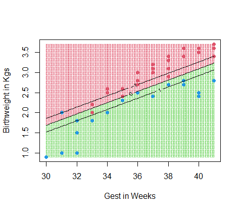 Support Vector Machine (SVM) attempts to separate sets of input data into groups. In the ideal situation, when the modelling data are easily separable, a simple decision border (a straight line or a flat hyperplane) can be established. In most situations however, the relationships between the input variables are complex, and the data require some form of transformation before a satisfactory decision border can be established. This transformation requires the use of a kernel. Although experienced mathematicians can derive kernels to suit a specific problem to be solved, most SVMs use on of the following 4 common kernels. The Linear kernel is the simple straight line or flat hyperplane, without any transformation. This is the simplest kernel, and are used when the data in the groups are eaily separable. The plot to the right demonstrates the results of training a SVM using a linear kernel. 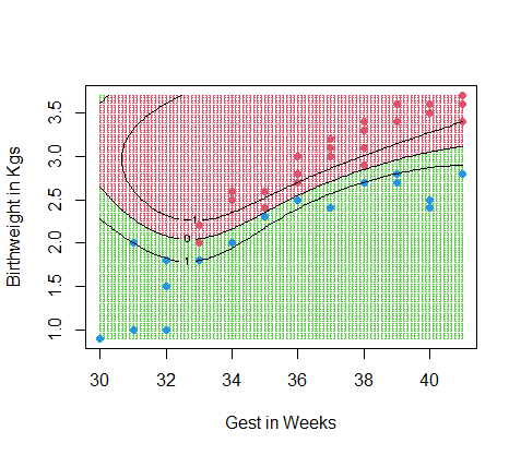Gaussian, also called Radial Function, abbreviated to Radial kernel uses a multi-dimensional Gaussian transformation to adapt the decision boundary to achieve the best possible separtion between the two groups. The kernel is often used, particularly when large number of input variables are involved, and the relationships between the variables complex or unknown. The use of the radial kernel required the user to specify the value gamma (γ). The higher the value, the more separations can be achieved. Too high a γ will cause the groups to break apart into meaningless individual islands, so some trial and error is required to determine the correct value. The default γ offered by R is 0.5, as shown in the plot to the left. This shows the 2 groups well separated, with no false negative, 1 false positive, 6 data points correctly classified but in the uncertainty zone. The remainders are clearly and correctly classified. This demonstrates the greater flexibility to make decisions according to the shape of the data, when compared with the Linear kernel. Although SVM with Radial kernel is the most flexible and commonly used kernel because of its great adaptability. it has the disadvantages of requiring long training time when the data is large and complex, and a tendency to overfit the training data, making the results less reproducible on other fresh sets of data. 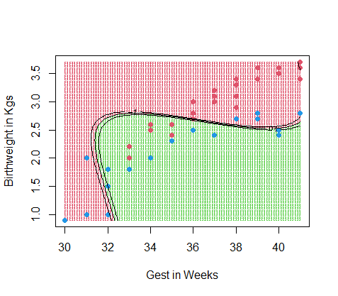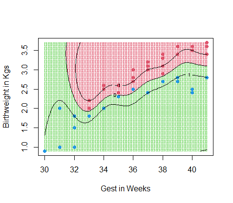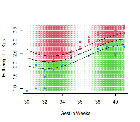Polynomial kernel uses a polynomial transformation of the decision border into curves with one or more peaks and troughs. The use of the polynomial kernel requires the user to specify the degree of polynomial transformation is defined. Degree of 1 results in a stright line or flat hyperplane. The greater the degree, the more complex the curves in the resulting decision border. The plot to the right used degree=3, which is the default value provided by R. Increasing the degree value training the current set of data failed to improve the fit, partly because the sample size is too small, the data not evenly distributed, and the line of separation does not have a polynomial shape. This example demonstrates how this kernel may fail when applied to unsuitable training data. 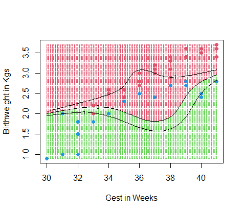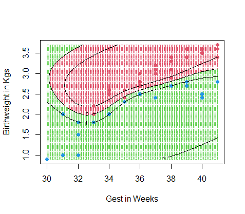Sigmoid kernel uses a sigmoidal transformation of the decision border, and is best used when the relationships between training variables are sigmoidal in shape, sich as logistic or probability values. As with the Polynomial kernel, sigmoid kernel has no advantage when used on unsuitable data, as shown in the plot to the right. Conclusions The Gaussian (Radial) is the most adaptable and tunable kernel one to use, particularly when the model involves numerous variable that have complex relationships. The Linear is the simplest and intuitively easy to understand kernel, but it lacks precision when the data contains numerous variables or have complex relationships. The Polynomial and the Sigmoid are useful only when the shape of the data is appropriate to the kernel Training Parameters A number of other parameters can be included during training, each will change the results, depending on the trainers preferences. R provides a good description of these parameters in its documentation https://www.rdocumentation.org/packages/e1071/versions/1.7-14/topics/svm, and the following are the ones used in the current example. Type = "C-classification" is used to separate data into groups, the most commonly used, and discussed on this page. The other types are for special purposes, and not covered here Cost defines how the data points near the decision border are used during training, and the width of the soft margin (the zone of uncertainty). If the data is clearly separable, Cost become irrelevant, as the hard margin can be established. Defining Cost is more important when the data in the different groups are close to or overlap each other The higher the cost, the wider the soft margin, and the more data points included in the zone of uncertainty. This means greater difficulty for the SVM to make a clear classification, but also that the SVM is less prone to false classification when used on other sets of data, as it is less likely to be overfitted to the training data The example on this page set Cost=10. Scale = "TRUE" or "FALSE" The 2 plots on the right show the difference The left plot is the results from Scale="False". All input data are used as presented. The difference in scaling (gestation 32-41, birthweight 2.0-4.0) may create instability in the decision border, as shown in the plot to the right. The right plot is the results from Scale="TRUE", and this is the default if Scale is not specified. All input variables are rescaled to similar values of mean=0 and SD=1 to stablize the relationship between variables, as shown in the plot to the left. This is particularly important when there are nore than 2 variables in the data set. An alternative: would use the option Scale="False", but have all input data pre-scaled to the same range (-1 to 1, 0 to 1, -4 to +4 SDs). The user can then have a known set of transformations for each input variable before the data is presented for training Gamma γ is the parameter associated with the Radial kernel, and it determines the complexity with which the decision border adapts to the training data. This is demonstrated by the 2 plots to the right, the left plot resulted from γ=0.2 and the right plot γ=0.8. It can be seen that increasing the γ value resulted in increasing the Radial Kernel's adaptability to the training data, reducing the number of data points that are wrongly classified or in the uncertainty zone. If not specified by the user, R sets the default value of γ=0.5 Degree is the parameter specific to the Polynomial kenrnel, and it dertermines the number of peaks and troughs in the decision border. Degree=1 results in the Linear kernel, and increasing degrees results in increasing complexity of the cirves. Output of the Trained Support Vector Machine The trained SVM procides the following information The vectors are the data points that are used to draw the Decision border.constant (offset) and the coefficients representing the line or the plane of the decision border D E F Contents of H:7 Explanation R Code C D E Contents of Explanation:80 Contents of R Code:81 Contents of C:82 Contents of D:83 Contents of E:84 Contents of I:8 Contents of J:9 Contents of K:10